In Edge Inspection, Input Drift Shows Up Before Accuracy Drops

EDGE AI

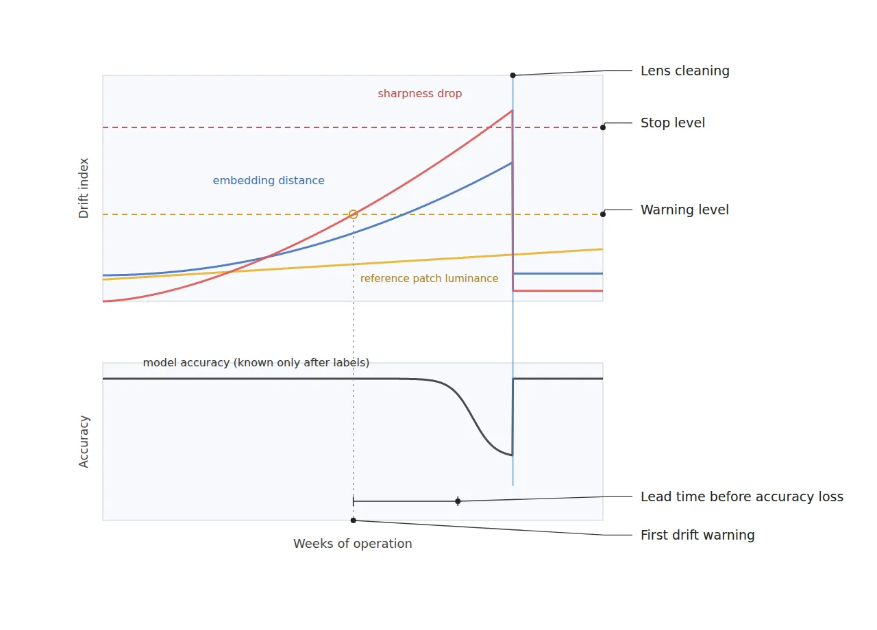
Reference-patch luminance and sharpness move before accuracy does. Set a per-frame p99 alarm and it fires once every 100 frames, so the alarms go on EWMA values.

On an edge device inspecting plated connector terminals at 15 μm/px, I calculated the cost of three indices (luminance, sharpness and embedding distance), their smoothing, and the warning and stop thresholds in turn.

About 11 min read

Performance loss in an edge inspection system usually starts quietly. A thin film of oil settles on the front of the lens, the LED output of the light drops little by little, and vibration turns the focus ring a hair. None of these changes a decision within a day, so the floor notices that something has changed only after overdetection or misses rise visibly. The lower the defect rate of a line, the slower ground-truth labels pile up, so thousands of parts pass before an accuracy drop can be confirmed, and the defects shipped in the meantime cannot be recalled.

The surface comes first. Plated metal terminals return light almost like a mirror, so under coaxial lighting flat faces image bright while the slopes of scratches and dents image dark. In return, small differences in machining grain direction and plating thickness shake brightness and sharpness, and the thresholds for the indices below have to be set with that wobble built in. Whether the thresholds hold under these reflection conditions cannot be guaranteed before a sample test.

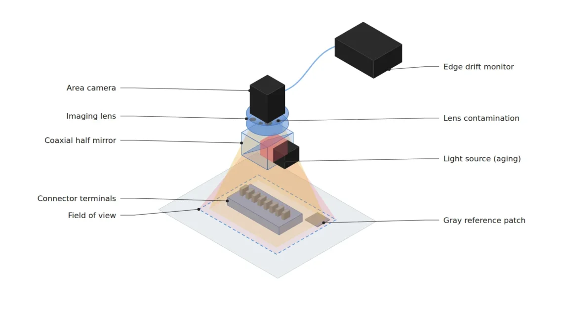
Here are the assumptions. A 2,448 × 2,048 px camera with 3.45 μm pixels and a 25 mm lens captures a 36.7 mm × 30.7 mm FOV at 15 μm/px from about 134 mm at the lens principal plane (a WD¹ of 120 mm or more secured). The light is coaxial illumination², and a matte gray reference patch of 64 × 64 px sits in a corner of the FOV. The smallest defect is a scratch 45 μm wide, and the device makes 5 decisions per second.

Accuracy moves in steps, input statistics in slopes

A trained model has some headroom against brightness changes and mild blur. Within the augmentation range of its training data, decisions hold while the input shifts a little, and then accuracy drops all at once when the headroom runs out. Mean luminance, by contrast, moves continuously from the start in proportion to the light output, and sharpness in proportion to the contrast the lens transfers. Input statistics show the headroom shrinking, while accuracy shows only the end result.

Seen at 15 μm/px, a 45 μm scratch is 3 px wide. If lens contamination widens the blur by just 1 px, a smear equal to a third of the defect width erodes the edge contrast. If the light weakens by 10 %, a defect with 30 gray levels of contrast shrinks to 27 levels in preprocessing with a fixed gray threshold, and where shot noise³ dominates, the signal-to-noise ratio also falls to √0.9 ≈ 0.95 times. The model still gets most decisions right at this stage, but its headroom is already shrinking. So what I watch is how far the input has moved from its distribution at training time, more than whether the model is wrong. Labels arrive late, but input statistics come with every frame.

One index for each cause

With one drift⁴ index per cause, three of them, mean luminance, sharpness and embedding⁵ distance, separate most optical degradation. Mean luminance catches light degradation, sharpness catches lens contamination and focus loss, and embedding distance catches distribution changes the first two do not explain. If only luminance drops, suspect the light; if only sharpness drops, the lens or focus; if both are fine and only the embedding distance grows, look first at a product or process change, so the combination of the three indices works directly as a diagnostic table.

The computation is cheap too. Shrinking a 2,448 × 2,048 px image to a quarter on each side gives 612 × 512 = 313,344 px, and the variance of Laplacian⁶ computed on it is negligible next to inference. The embedding reuses the feature vector the backbone of the decision model has already computed, so no extra inference run is needed.

Luminance is measured on a 64 × 64 px matte gray reference patch fixed in a corner of the FOV, away from the product area. It separates the color and gloss variation of the product itself from light degradation, and the moment one reference patch enters the FOV, light degradation and product variation become different numbers. In my case the patch position goes on the drawing at installation, so the same pixel area is read even after the camera is remounted.

Per-frame p99 alarms fire once every 100 frames

Put the alarm threshold on individual frame values and the alarm fires even when nothing is wrong. A rule that warns above the p99 of the good-part distribution trips once every 100 frames by definition, and on a device making 5 decisions per second that is once every 20 seconds. An alarm that is always ringing ends up switched off, and a switched-off alarm reports no degradation.

So all three indices carry their thresholds on EWMA⁷-smoothed values. With λ = 0.05 the smoothing length resembles a moving average of about 39 frames, and the wobble of the value shrinks to √(λ ÷ (2 − λ)) ≈ 0.16 times that of the raw index, so slow slopes of a few percent rise above the noise. NIST’s description of EWMA control charts notes that λ is usually set between 0.2 and 0.3, but since the goal is slow degradation over weeks, I use the longer 0.05. Sudden failures are caught late in exchange, so per-frame anomaly decisions handle those separately.

The thresholds come in two levels. The warning schedules cleaning or a check when the headroom starts to shrink, and the stop holds decisions just before decision reliability collapses and flags the parts in that stretch for re-inspection. Baselines come from the statistics of a period of stable running on good parts, never from the moment of installation, and after lens cleaning or light replacement, whether the three indices return to baseline is recorded as the effect of the maintenance.

Embedding distance starts by cutting dimensions

Defining embedding distance as the Mahalanobis distance⁸ to the good-part distribution requires the covariance matrix of the good-part features and its inverse. With 512-dimensional backbone features and 500 good parts, the rank of the sample covariance is at most 499, so the inverse does not exist. The calculation may appear to run, but along directions with tiny eigenvalues the distance blows up absurdly, and alarms fire on the wrong frames.

So I cut the features down to about 32 dimensions with PCA⁹ before measuring distance. At 32 dimensions the covariance has 528 independent elements and there are 15.6 good parts per dimension, so the estimate is stable, and where cutting dimensions is hard, shrinkage estimation of the covariance is another route. The warning and stop thresholds are set at the p99 and p99.9 of the measured distribution traced by the EWMA during stable running, in place of chi-square values that assume a normal distribution.

Thresholds worked back from a 45 μm scratch

Defect size, optical setup and the thresholds of the three indices are gathered in one table. The luminance and sharpness numbers are starting points, readjusted by measurement on site.

Item	① Minimum defect size	② Optical setup · WD	③ Algorithm parameters
Terminal scratch	Width 45 μm = 3.0 px (15 μm/px)	2,448 × 2,048 px, 3.45 μm pixels, 25 mm lens, FOV 36.7 × 30.7 mm, coaxial light, WD 120 mm or more (object distance about 134 mm from the principal plane)	Sharpness: variance of Laplacian on a quarter-size image (612 × 512 px), warning −15 %, stop at the measured value for 1 px of blur
Terminal dent	Diameter 75 μm = 5.0 px	Matte gray reference patch of 64 × 64 px in a corner of the FOV	Reference luminance: warning −5 %, stop −10 %
Distribution change	Changes the other two indices do not explain	Backbone features reused (no extra inference)	Embedding distance: Mahalanobis in 32 PCA dimensions, warning at EWMA p99, stop when EWMA exceeds p99.9 for 20 frames in a row
Smoothing	At 5 decisions per second	Return to baseline recorded after light replacement and lens cleaning	EWMA λ = 0.05 (about 39 frames, wobble 0.16 times)

The cell most likely to be loose in this table is the sharpness stop threshold. At 15 μm/px a 45 μm scratch is exactly 3.0 px, so just 1 px (15 μm) more blur can push it below the detection floor, and a statistically chosen number like −30 % knows nothing of that geometry. So at installation I deliberately turn the focus ring in small steps, measure the sharpness value at the point where the scratch edge widens by 1 px, and use that value as the stop threshold. Drift thresholds are not set by statistics alone; they are worked back from how many pixels the minimum defect occupies.

When tracking output accuracy directly is better

Some processes are better served by the opposite approach. If the defect rate is high and dozens of re-inspection results come back every hour, tracking output accuracy directly makes the more accurate monitor. On high-mix lines with frequent product changes, the embedding baseline changes with each product, so where per-product baselines are hard to maintain, running only reference luminance and sharpness is the realistic choice. And on equipment whose calibration interval is well shorter than the drift speed, constant monitoring gains little.

Drift monitoring is a function that reports optical degradation; it does not correct it. Normalizing luminance in software to flatten the indices makes things look stable while the loss in resolution and signal-to-noise ratio stays, and the fix comes from hardware actions such as lens cleaning, light replacement and refocusing. On plated terminals, diffuse components and machining variation can shake the sharpness index itself, so the thresholds above cannot be guaranteed before a sample test.

Field Note

If overdetection on an edge inspection system creeps up over a few weeks, I trace the sharpness and reference luminance trends in the stored images before considering retraining. Optical changes such as a thin oil film on the lens front can leave traces in the input images before accuracy drops. When an index crosses the EWMA warning line, cleaning or a check comes first, and after cleaning I confirm that the three indices return to baseline. The stop threshold is set per machine by measurement, blurring the focus on purpose.

Field Checkpoints

Before switching on drift monitoring, I check that the items below are in place. The reference patch, the thresholds and the records all have to exist for an alarm to mean anything.

• Is a WD of 120 mm or more secured by measurement, including the coaxial light housing and the reference patch bracket? (object distance about 134 mm from the principal plane)
• Have you measured on good samples how much the machining grain and plating variation of the terminals shake the sharpness index?
• Is luminance drift measured on a fixed reference patch in the FOV in place of the product area?
• Are the warning and stop thresholds set on EWMA values instead of frame values? (a per-frame p99 alarm fires once every 100 frames)
• Is embedding distance computed in PCA-reduced dimensions, with baselines taken from good-part statistics during stable running?
• Was the sharpness stop threshold set from the measured value at a 1 px edge widening, and is the return of the indices recorded after cleaning or replacement?

Frequently Asked Questions

If accuracy is sampled periodically, is drift monitoring still needed?

Confirming that misses have risen on a line with a 0.1 % defect rate takes dozens of defects, and gathering 50 of them means 50,000 parts passing. Meanwhile input statistics accumulate with every frame and show the same degradation much earlier. I use both, with the input indices raising the alarm and accuracy sampling confirming whether the alarm was right.

What if the reference patch gets dirty?

The reference patch catches the same dust as the lens, so when its luminance drops, light degradation and patch contamination have to be told apart. I put the patch on the cleaning checklist and compare the luminance right after cleaning with the new baseline to check separately whether the light output itself has dropped.

Glossary

• [1] WD working distance
  The distance from the front of the lens to the surface under inspection. The roughly 134 mm in the text is a thin-lens object distance from the lens principal plane; the distance from the lens front comes from the lens drawing. ↩
• [2] Coaxial illumination coaxial light
  Lighting that sends light down along the lens optical axis through a half mirror. Flat metal faces image bright and tilted scratches image dark. ↩
• [3] Shot noise shot noise
  Noise from the random arrival of light quanta. It scales with the square root of the signal, so 10 % less light lowers the signal-to-noise ratio by about 5 %. ↩
• [4] Drift drift
  The gradual movement of input image statistics away from their distribution at training time. ↩
• [5] Embedding embedding
  The feature vector a model backbone produces to summarize one image. Similar images give nearby vectors. ↩
• [6] Variance of Laplacian variance of Laplacian
  The variance of an image after a second-derivative filter; the sharper the edges, the larger it is. It expresses lens contamination or focus loss as one number. ↩
• [7] EWMA exponentially weighted moving average
  A moving average that adds λ times the new value to 1 − λ times the previous smoothed value. The smaller λ, the longer the smoothing. ↩
• [8] Mahalanobis distance Mahalanobis distance
  A distance that takes into account the directions and sizes of a distribution’s spread. It needs the inverse of the covariance matrix. ↩
• [9] PCA principal component analysis
  A method that cuts dimensions by picking, in order, the directions along which the data spreads most. ↩

References

• NIST, 6.3.2.4. EWMA Control Charts (gives the standard deviation of the EWMA statistic as √(λ ÷ (2 − λ)) × s, a control limit factor k usually of 3, and λ usually between 0.2 and 0.3)
• Formulas: pixel resolution = FOV ÷ pixel count, defect width (px) = defect width ÷ pixel resolution, shot-noise signal-to-noise ratio ∝ √signal, EWMA z_t = λx_t + (1 − λ)z_t−1, equivalent moving average length = 2 ÷ λ − 1, EWMA standard deviation ratio = √(λ ÷ (2 − λ)), per-frame p99 false alarm interval = 1 ÷ 0.01 frames, rank of sample covariance ≤ sample count − 1, magnification m = sensor width ÷ FOV width, object distance = f × (1 + 1/m)
• Assumptions: 2,448 × 2,048 px camera (3.45 μm pixels), 25 mm lens, FOV 36.7 × 30.7 mm, minimum defect 45 μm, defect contrast 30 gray levels, 10 % light loss, 5 decisions per second, 512-dimensional backbone features, 500 good parts for the baseline, 32 PCA dimensions, defect rate 0.1 %

Related reading — It Worked on the Server, So Why Does Accuracy Drop on the Edge? · When an LED Light Dims, Yesterday’s Threshold Misses Today’s Defect · Why an Average Latency Inside the Deadline Is Not Safe