A Board at 0.5 m/s Leans 15 mm Under a Rolling Shutter

OPTICS

On the same board, a rolling shutter leans 15 mm and a global shutter smears 50 μm.

Fix the sensor and the lens, change only the shutter, the color and the cable, and each camera type shows its own way of leaving a defect in the picture.

About 14 min read

Photograph a board passing at 0.5 m/s with a rolling shutter camera and the top row and the bottom row of the picture end up 15 mm apart. In a 100 mm field that is 614 pixels, which is enough to make the whole picture useless for finding a 50 μm scratch. The surface is green solder mask, close to matte, and I assume its reflectance¹ is middling. Smooth, specular patches appear only where the copper pads are exposed. The sensor (4,096×3,000 px, 3.45 μm pixels) and the lens (25 mm) are also assumptions for the calculation, and with that pair one pixel covers 24.41 μm and the WD² is 201.9 mm.

The split between area scan and line scan is settled by now. Inside area scan alone, the camera type still divides again by how the shutter opens, how color is read, and which cable carries the picture. The first two decide whether the defect stays in the picture, and the last decides whether the surviving picture reaches the computer. If one of them is off, the missed scratch is packed into a good-parts box, ships, and comes back as a failure inside the customer’s device. The sensor and the lens stay fixed below, and only those three change on the same board.

Which camera type keeps a 50 μm defect in the picture and delivers it to the computer?

A rolling shutter stitches together rows taken at different moments

A rolling shutter³ opens and reads the sensor rows one after another from top to bottom. VA Imaging explains that each row is exposed at a different time, so a fast-moving object comes out distorted. The size of the distortion is set by how long one full readout takes. If 3,000 rows are read at 10 μs per row (an assumption), one picture takes 30 ms. The readout speed is an assumption, and the real value is an item to confirm in the sensor data sheet.

Picture a window blind raised one slat at a time from the bottom while a person walks past outside. The person seen through the upper slat is on the left, the person seen through the lower slat is on the right, and in the stitched picture the person leans sideways.

Say the board moves sideways at 0.5 m/s and the rows are read from top to bottom. In 30 ms the board travels 0.5 m/s × 30 ms = 15 mm. One pixel is 24.41 μm, so that is 614.4 pixels and 15 % of the field. A square part is recorded as a parallelogram.

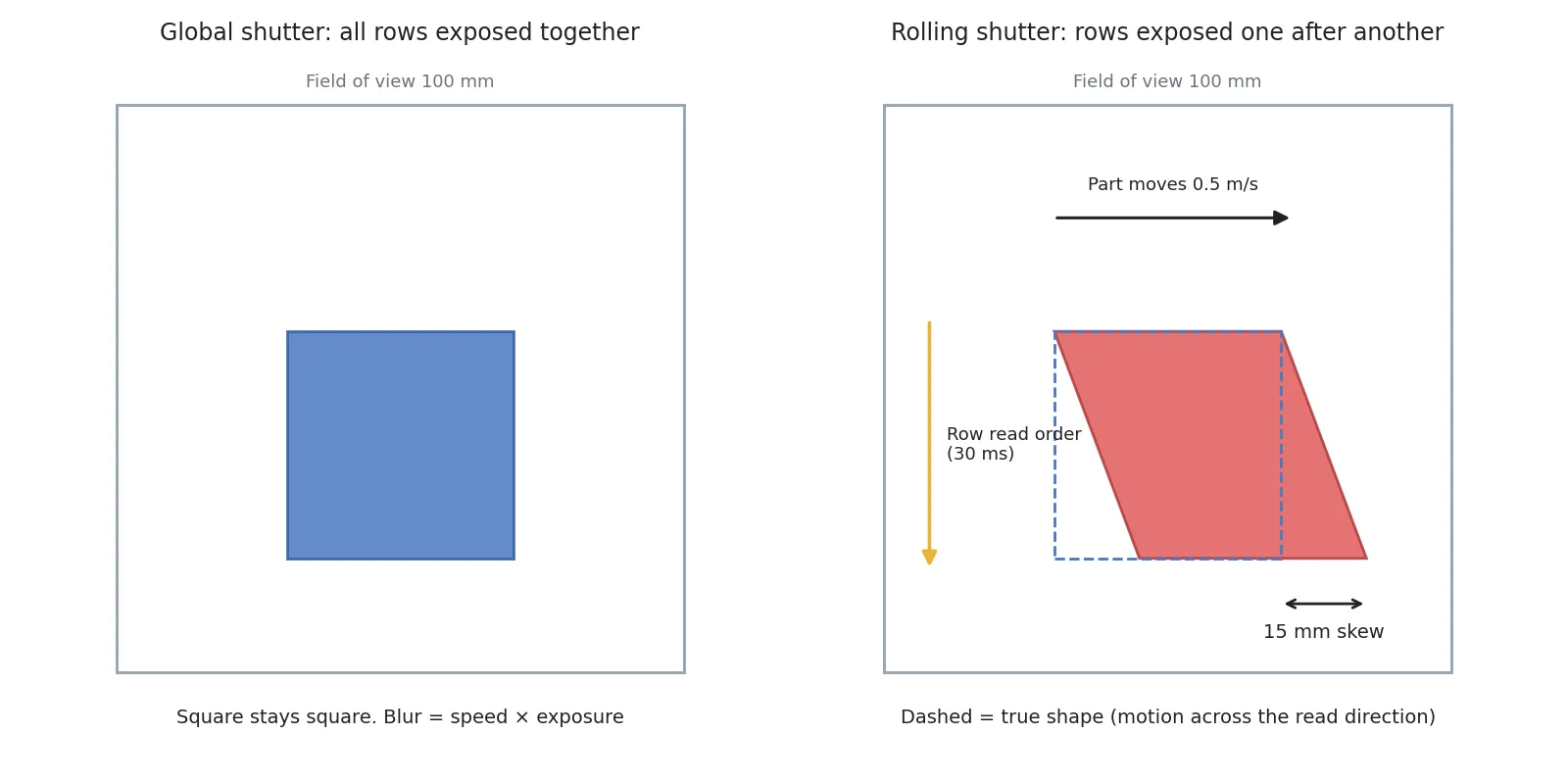
Look first at the top edge, where the dashed square and the red parallelogram meet. The top row sits in place and only the bottom row is pushed 15 mm to the right. Nothing in this shift is smeared, so it stays sharp, yet the position is wrong and no dimension can be measured from it. Undoing it needs the read time of every row, which is another value to confirm in the data sheet, and before I plan to fix it in software I look for a way to stop it on the camera side.

Motion is not the only problem. VA Imaging reports that under a 50 Hz fluorescent lamp (10 ms period) a 5 ms exposure puts horizontal stripes on a rolling shutter picture and none on a global shutter picture. In a plant with a flickering ceiling light, the camera gets one more item on its checklist.

Switching to a global shutter still leaves the exposure to set the smear

A global shutter⁴ exposes every row at the same moment, so the parallelogram disappears. Smear stays. With a 100 μs exposure (an assumption) and the board moving at 0.5 m/s, 0.5 m/s × 100 μs = 50 μm smears, the same as the width of the scratch being sought. To hold the smear within one pixel (24.41 μm), the exposure has to be 24.41 μm ÷ 0.5 m/s = 48.8 μs or less. So people who use a global shutter reach for the exposure control as well. With a 20 μs strobe⁵ pulse (an assumption) the smear drops to 10 μm, less than half a pixel.

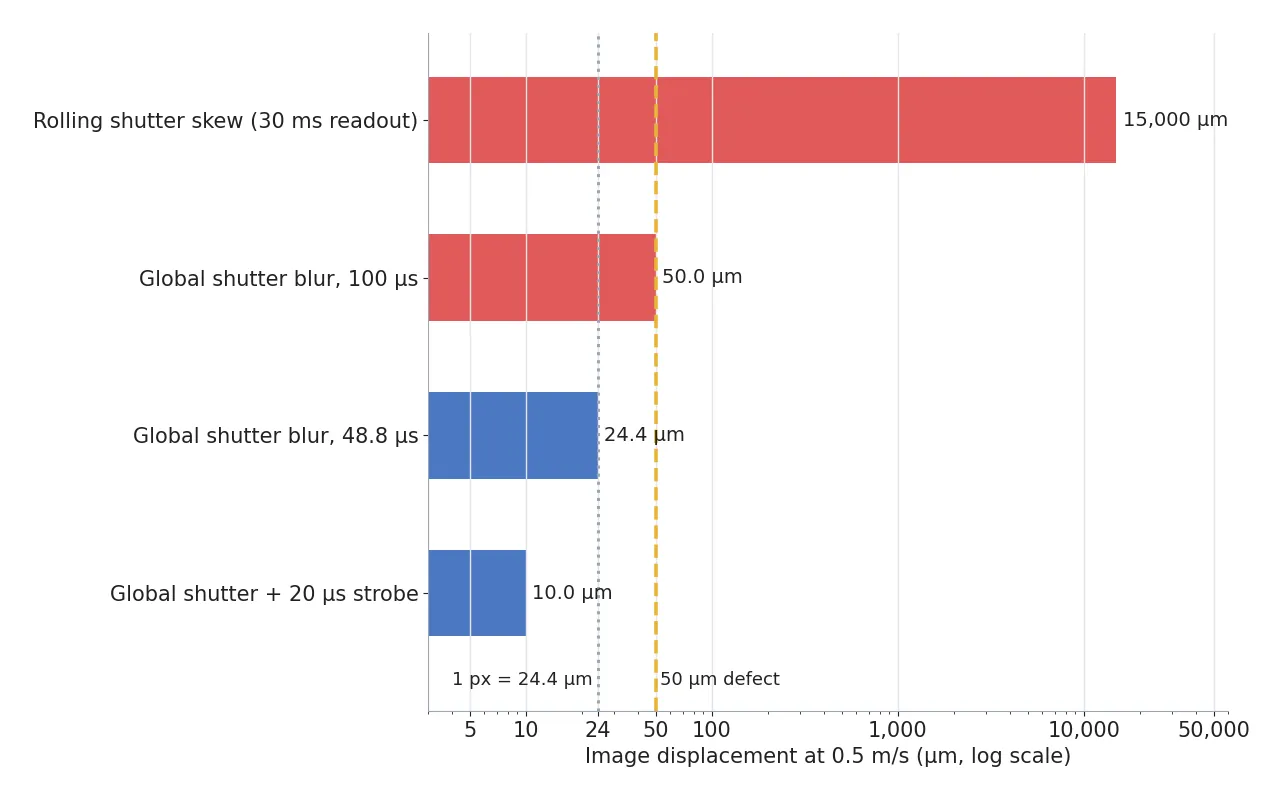
Look first between the gray dotted line (one pixel) and the yellow dashed line (the 50 μm defect). The 100 μs global shutter bar touches the yellow line exactly, and the 15,000 μm rolling shutter bar only fits when the axis is logarithmic. Three orders of magnitude separate the two.

There is a cheap way to use a rolling shutter too. VA Imaging says a flash fired at the moment the exposure of every row overlaps removes the distortion, and adds that when the exposure is too short and the readout too long the rows do not overlap and the strobe will not fire. With a 30 ms readout and a 35 ms exposure (an assumption), the overlap is 5 ms and a 20 μs pulse fits inside it. The sensor, however, also collects room light for the full 35 ms. Against a 20 μs strobe, ambient light enters 35 ms ÷ 20 μs = 1,750 times longer, so this route works only if the stage can be shaded dark.

VA Imaging also points out that a global shutter sensor is larger at the same resolution and costs more. The same page says rolling shutter cameras are more common above 1.6 MP. The near-infrared illumination calculation for a global shutter sensor has its own article, Changing the Sensor Means Recalculating the Illumination.

Monochrome measures light and color guesses it

The sensor in a color camera does not know color either. The Imaging Source explains that a sensor only counts photons, so a Bayer pattern⁶ with a red, green or blue filter over each pixel is used almost without exception. Turning it into a picture with visible color needs debayering⁷, which fills the two missing colors from neighboring pixels, and that interpolation softens thin edges and lowers the real spatial resolution.

In numbers it looks like this. In a Bayer pattern (RGGB assumed) the red filter sits on every second pixel in both directions, so seen in red alone the sample spacing is 2 pixels, or 2 × 24.41 μm = 48.83 μm. A 50 μm scratch spans 1.02 red samples. If, as in the earlier calculation, two samples must be covered to count as identified, the smallest size identified in red or blue alone is 97.66 μm, while the monochrome version of the same sensor reaches 48.83 μm.

The amount of light drops as well. A pixel under a red filter blocks green and blue photons, so the quantum efficiency of the whole sensor falls sharply, according to The Imaging Source. The same text gives no figure, so how much it falls is an item to confirm in the spectral curve of the data sheet. Monochrome can shorten the exposure under the same light, it says, which favors keeping to a short exposure limit like the 48.8 μs above.

Color is rarely the defect on this board. The scratch on green solder mask and the marks on a copper pad show up as differences in brightness. The Imaging Source gives an example in which a red LED turns a green circuit board black and gives a monochrome camera strong contrast, and I would start with a monochrome camera and colored light before a color camera. For inspections where color is the defect, such as color-coded fuses or label printing, I pick color from the start. How the two split on the copper pad spots that wash out to white cannot be guaranteed before a sample test.

Color also brings payload. RGB debayered inside the camera sends three 8 bit values per pixel, three times monochrome, while raw Bayer 8 bit equals monochrome but leaves the interpolation to the computer. That factor of three carries into the cable calculation.

Bits per picture choose the cable

A water pipe cannot deliver more water at once than its width allows. A picture likewise cannot be sent faster than the number of bits the cable carries per second, its bandwidth⁸. At 4,096×3,000 px (12.29 MP) and 8 bit per pixel, one picture is 98.3 Mbit. At 30 fps monochrome needs 2.95 Gb/s, and the same picture sent as RGB 24 bit needs 8.85 Gb/s.

Divide the nominal rates in the Edmund Optics table by this picture size and the frame-rate ceiling appears. GigE at 1 Gb/s gives 10.2 fps, USB3 and 5GigE at 5 Gb/s give 50.9 fps, Camera Link at 6.8 Gb/s gives 69.2 fps, 10GigE gives 101.7 fps, and CoaXPress⁹ CXP-12 at 12.5 Gb/s gives 127.2 fps. With RGB 24 bit everything drops to a third, GigE to 3.4 fps and 10GigE to 33.9 fps. The effective rate after protocol overhead is lower, so the real value is an item to confirm in the camera data sheet.

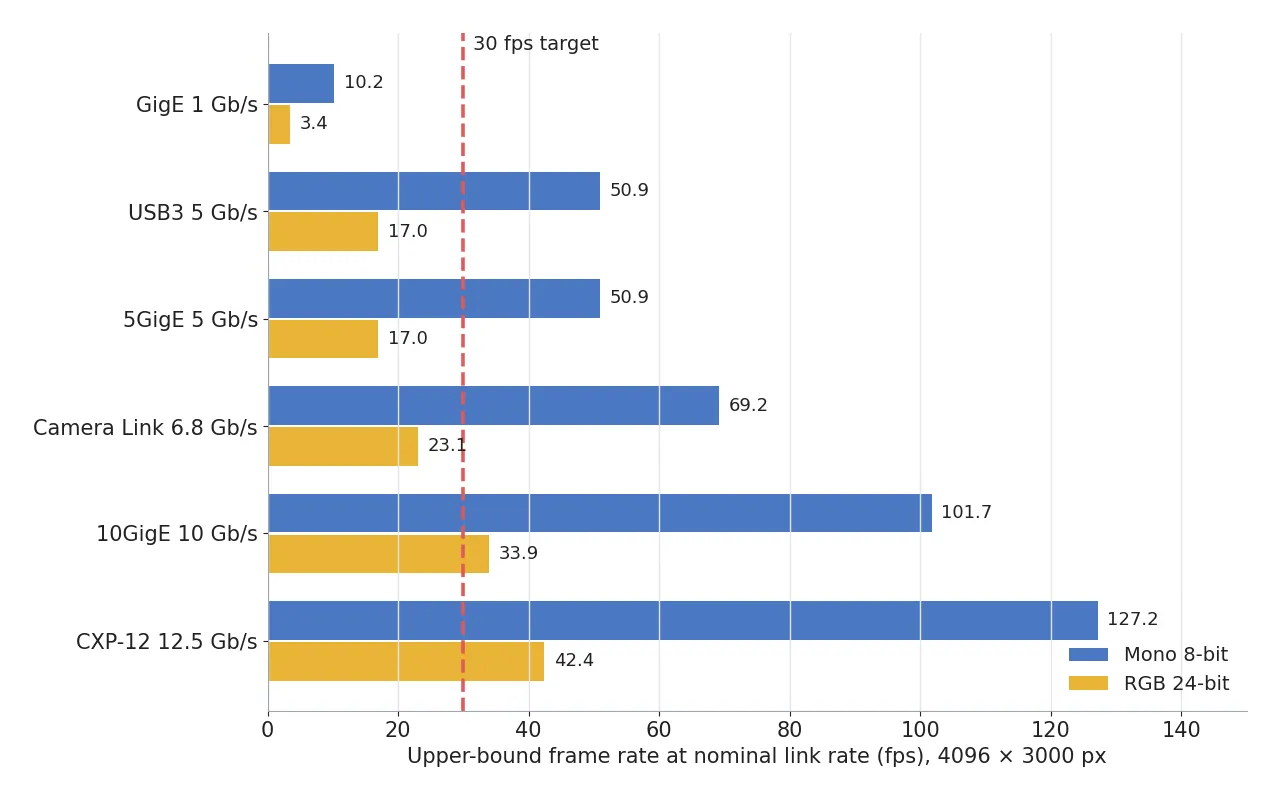
Look first at the red 30 fps dashed line. In monochrome only GigE stays left of it, and in RGB 24 bit only 10GigE and CoaXPress cross it. Distance comes with it. In the Edmund Optics table USB3 has a recommended 3 m, GigE and 10GigE 100 m, Camera Link 10 m and a mandatory capture board, and CoaXPress runs beyond 100 m at 3.125 Gb/s. If the control cabinet is far from the stage, USB3 drops out of the candidates first.

Line scan gets the same calculation. Reading 8,192 px at 8 bit and 40.96 kHz gives 2.68 Gb/s, above the 1 Gb/s of GigE. The bandwidth design per interface is worked out in a separate article, Camera Interface Bandwidth Determines Resolution.

Five camera types on one data sheet

Five rows with the sensor and lens fixed and only the shutter and the color changed. The cable does not change by row, and the transfer calculation above attaches to each one as it is. Read each row in the order ①②③, and the assumed values are the ones stated in the earlier sections.

Camera type	① Smallest identifiable size	② Optical setup · WD	③ Algorithm parameters · In plain words
Rolling shutter, moving sample	48.8 μm (2 px, 24.41 μm/px). But it leans 15 mm (614 px)	25 mm lens, WD 201.9 mm (confirm in the data sheet), continuous light	Row readout 30 ms (assumed) times sample speed exceeds the position tolerance. Not suited to a moving board
Rolling shutter + strobe	48.8 μm. Smear 10 μm for a 20 μs strobe	WD 201.9 mm, pulse inside the 5 ms overlap of a 35 ms exposure, dark shade needed	Ambient light enters 1,750 times longer than the pulse. Confirm trigger delay in the data sheet. A dark enclosure is the condition
Global shutter	48.8 μm. Smear 50 μm at 100 μs, within one pixel at 48.8 μs or less	WD 201.9 mm, larger sensor and higher price at the same resolution (VA Imaging)	Exposure ceiling 48.8 μs, smear 10 μm with a 20 μs strobe. No lean, only smear
Monochrome	48.8 μm (2 px)	WD 201.9 mm, colored light such as a red LED builds contrast on a green board	One 8 bit channel, 2.95 Gb/s at 30 fps. Color is dropped and only brightness is measured
Color (Bayer)	97.66 μm in red or blue alone, twice monochrome	WD 201.9 mm, white light, confirm glossy areas on samples	Debayering needed, 8.85 Gb/s at 30 fps for RGB 24 bit. Color is filled in by guessing

What shows first across the five rows is that the sensor and lens are the same, so the WD (201.9 mm) and the smallest identifiable size (48.8 μm) are the same everywhere. The camera type decides three things: lean and smear in motion, color samples, and transfer volume. A different approach wins under some conditions. If the sample stands still while it is photographed and the lighting is steady, one rolling shutter color camera is better on both price and color information. When the assumed values in the table (10 μs per row, 100 μs exposure, 20 μs strobe) are replaced by real specifications, every row must be recalculated, and the result cannot be guaranteed before a sample test.

Three lines for the data sheet and who pays

The order is short. Write down first whether the sample moves, whether color is the defect, and how many meters the picture travels to the computer, then match the sensor and lens and confirm the WD. In my own data sheet I would put the sample speed and the exposure ceiling on the first line in place of a model name. The calculation for choosing the vision type itself is in the article comparing six vision types.

The sensor technology comes last. In the Edmund Optics comparison table CMOS has lower power consumption and cost and higher speed, while CCD has higher uniformity and fill factor. Recent high-end CMOS can beat a comparable CCD, yet low-end CMOS with pixels smaller than about 3 μm is still outperformed by CCD. The 3.45 μm pixel assumed here sits just above that line.

The job that makes this choice is the machine vision engineer, and a person who can put the shutter, the color and the cable into a single calculation finishes a conversation on site quickly. For those funding the equipment, the global shutter sensor costs more (VA Imaging) and Camera Link requires a capture board (Edmund Optics), and that is where the money shows. A rolling shutter and GigE cost less, in return for keeping the sample still or matching a strobe. This article explains technology and is not investment advice. See our Disclaimer.

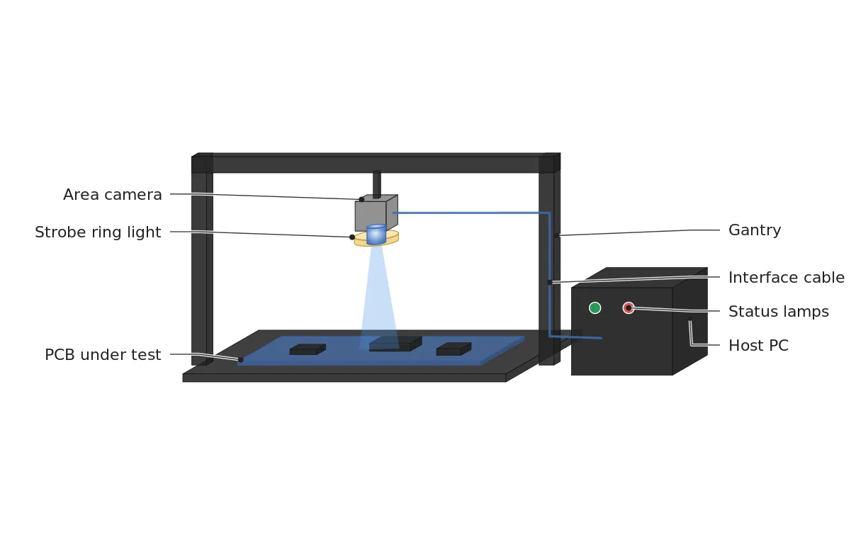
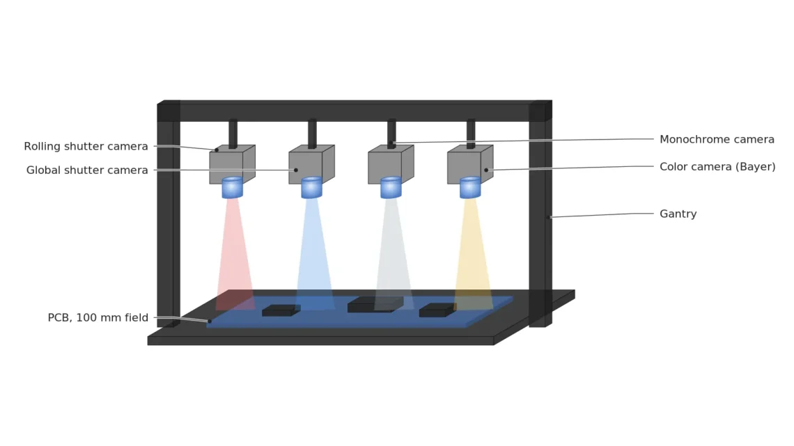
The figure collects this calculation on one station. The camera stands at a WD of 201.9 mm with a strobe ring around the lens, and the interface cable runs down the gantry column to the host PC. The cable length is the dimension the figure does not show, and beyond the recommended 3 m of USB3 the PC has to move.

Field Note

On a new setup I first photograph the board standing still to make a reference picture, then pass it through at 0.5 m/s and measure the offset between the top row and the bottom row with a ruler. A value near 15 mm sends me to the readout speed first, and a value near 0 sends me on to the smear. I hold the exposure to 48.8 μs or less and set a picture with the strobe on beside one with it off. For the copper pad spots that wash out to white, I take one monochrome and one color picture under the same light and compare them.

Field Checkpoints

Turning that check into data sheet lines leaves the following seven.

• Is the WD from lens to board top, 201.9 mm (25 mm lens, 14.13 mm sensor width assumed), still secured after adding the fixture and the strobe ring? (does room remain for lamps and hands)
• Is the sample speed times the row readout time (0.5 m/s × 30 ms = 15 mm) inside the position tolerance? (if it exceeds it, does the setup have to move to a global shutter or a strobe)
• Is the exposure at or below the one-pixel smear limit of 48.8 μs? (can the strobe pulse be set to 20 μs)
• If a strobe is used with a rolling shutter, does the pulse land inside the overlap of all rows (35 ms − 30 ms = 5 ms) and is ambient light shaded out? (is there room to put up a dark shade)
• Is color the defect, or does a brightness difference suffice? (if brightness, is starting with monochrome and colored light acceptable)
• Does the required transfer (monochrome 2.95 Gb/s, RGB 8.85 Gb/s at 30 fps) fit inside the effective rate of the chosen interface? (does the cable reach within USB3 at a recommended 3 m or GigE at 100 m)
• Have specular spots such as copper pads and solder been checked on sample images? (is the result left unstated until the calculation meets a sample)

Glossary

• [1] Reflectance reflectance
  The share of the light reaching a surface that comes back off it. White paper is high and black cloth is low. ↩
• [2] WD working distance
  The distance from the lens to the top of the part being inspected. The text calculates it with a thin-lens approximation from the principal plane, and the reference plane a maker uses has to be checked in the data sheet. ↩
• [3] Rolling shutter rolling shutter
  A method that exposes and reads the sensor rows one after another from top to bottom. Each row is captured at a different moment. ↩
• [4] Global shutter global shutter
  A method that exposes every pixel of the sensor at the same moment. A moving object keeps its shape. ↩
• [5] Strobe strobe
  A light that turns on for a very short time. How long it stays on is how long motion can smear in the picture. ↩
• [6] Bayer pattern Bayer pattern
  A layout that puts one red, green or blue filter over each pixel. A single pixel measures the light of one color only. ↩
• [7] Debayering debayering, demosaicing
  A calculation that guesses the two missing colors at each pixel from the values of its neighbors. Because it is a guess, thin edges get softer. ↩
• [8] Bandwidth bandwidth
  The number of bits a cable can carry in one second. The bits of one picture times the pictures per second must stay below it. ↩
• [9] CoaXPress CXP
  A camera interface that sends images over coaxial cable. CXP-12 in the text carries up to 12.5 Gb/s per cable. ↩

References

• VA Imaging, Rolling Shutter vs Global Shutter (per-row exposure time, distortion of moving objects, fluorescent stripes, strobe conditions, sensor size and price), accessed October 14, 2026
• The Imaging Source, Monochrome vs. Color Cameras in Machine Vision (Bayer pattern, debayering and resolution, quantum efficiency, payload, colored light example), accessed October 14, 2026
• Edmund Optics, Camera Types and Interfaces for Machine Vision Applications (speed and cable length per interface, CCD and CMOS comparison table), accessed October 14, 2026
• Formulas: pixel footprint = field ÷ horizontal pixel count, rolling shutter lean = sample speed × row count × readout time per row, smear = sample speed × exposure time, Bayer sample spacing for one color = 2 × pixel footprint, bits per picture = horizontal pixels × vertical pixels × bit depth, frame-rate ceiling = nominal rate ÷ bits per picture