Must You Wait Until Model Accuracy Drops? — Monitoring Input Distribution Drift in Edge Inspection

EDGE AI / ALGORITHM

The performance degradation of an edge inspection system usually begins quietly. A fine film of oil settles on the front of the lens, the light output of the illumination LEDs drops little by little, and vibration turns the focus ring by a tiny amount. None of these changes the decision results in a single day. So the site notices that “something has changed” only after the model’s over-detection or missed detection has visibly increased.

Left unaddressed, the cost piles up in two directions. Tilting toward missed detection lets defects escape, and tilting toward over-detection increases the scrapping of good parts and re-inspection. What is more troublesome is that the lower the defect rate of a line, the less the model accuracy can be measured in real time. Confirming an accuracy drop without ground-truth labels requires thousands of parts or more to pass, and the defects that escape in the meantime cannot be recalled.

The solution is to monitor not the output of the model but the input of the model. Lens contamination, illumination degradation and focus drift leave traces in input statistics such as mean luminance, a sharpness metric and embedding distance before they affect accuracy. These metrics need no labels and can be computed lightly at the edge on every frame.

Accuracy becomes visible only after waiting for labels, but input statistics speak on every frame.

1. Why Optical Degradation Shows Up in Input Statistics Before Accuracy

Point. Model accuracy responds to degradation in a step-like way, while input statistics respond in a continuous way.

Reason. A trained model has a certain margin against brightness changes and mild blur. Within the augmentation range of the training data, the decision holds even if the input changes a little. But the moment the margin is used up, accuracy falls sharply. Mean luminance, by contrast, moves continuously from the start in proportion to illumination output, and the sharpness metric in proportion to the contrast transfer characteristics of the lens. In other words, input statistics show the process of the margin being used up, while accuracy shows only the result once it is exhausted.

Example. Viewing a 45 µm scratch on a connector terminal at 15 µm/px, the defect width is 3 px. If lens contamination widens the blur by just 1 px, a spread equal to one third of the defect width erodes the edge contrast. If the illumination weakens by 10%, a defect with a contrast of 30 gray levels shrinks to 27 gray levels in preprocessing that uses a fixed gray-level threshold (design assumption). The shot-noise-based SNR also drops by a factor of √0.9 ≈ 0.95. At this stage the model still gets most cases right, but its margin is already shrinking.

Point. Therefore the target of monitoring should be not “is the model wrong” but “how far has the input moved from the distribution at training time”.

2. Three Drift Metrics Computed Lightly at the Edge

Point. One drift metric per cause, three in total, mean luminance, sharpness and embedding distance, can distinguish most optical degradation.

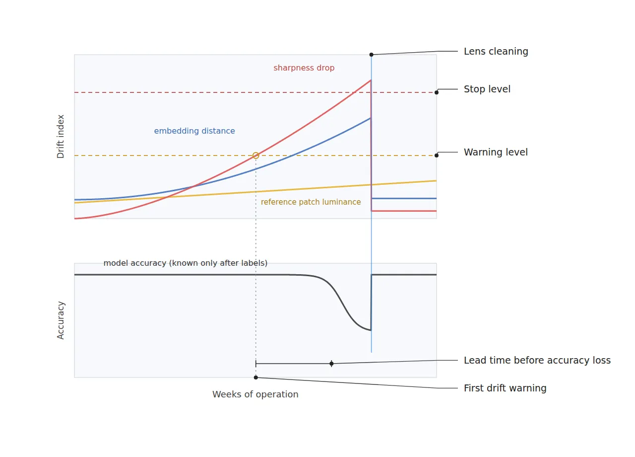
Reason. Mean luminance catches illumination degradation, the sharpness metric catches lens contamination and focus drift, and embedding distance catches every distribution change the other two cannot explain. The compute cost is also small. Mean luminance is a single summation, and for sharpness the Laplacian variance of a downscaled image is enough. The embedding reuses the feature vector already computed by the backbone of the decision model, so no additional inference is needed. What matters is measuring luminance not on the product area but on a fixed reference patch in the corner of the FOV. This keeps the color and gloss variation of the product itself from mixing with illumination degradation.

Example. Downscaling a 2448 × 2048 px image to 1/4 horizontally and vertically gives 612 × 512 = 313,344 px, and the cost of computing the Laplacian variance on it is negligible compared with inference. The reference patch is a 64 × 64 px matte gray patch, and only its mean luminance is computed. Embedding distance is defined as the Mahalanobis distance to the feature distribution of 500 good-part images. Smoothing all three values with an EWMA (exponentially weighted moving average, λ = 0.05) has the same effect as a moving average of about 39 frames.

Point. The combination of the three metrics becomes a cause diagnosis table. If only luminance drops, suspect the illumination; if only sharpness drops, the lens or focus; and if both are normal but only the embedding distance grows, suspect a change on the product or process side.

The moment a single reference patch is placed in the FOV, illumination degradation and product variation become different numbers.

3. Alarm Thresholds — Separating Warning from Stop

Point. Drift alarms must have two levels, warning (inspection request) and stop (decision hold), so that the site does not ignore them.

Reason. With only one threshold, setting it sensitively causes frequent false alarms that get ignored, and setting it loosely makes it ring after accuracy has already dropped. The warning schedules cleaning or inspection at the point the margin starts to shrink, and the stop halts the line just before decision reliability collapses. The reference values for the thresholds should be taken not right after installation but from the statistics of a period of stable operation with good parts.

Example. As design assumptions, reference patch luminance triggers a warning at −5% from the reference and a stop at −10%. Sharpness triggers a warning at −15% and a stop at −30%. Embedding distance triggers a warning when it exceeds the p99 of the good-part reference distribution, and a stop when exceeding p99.9 continues for 20 consecutive frames. On a stop, the decision is held and the parts of that interval are flagged for re-inspection. After lens cleaning, check that the three metrics return to their reference values and record the effect of the maintenance.

Point. Drift monitoring is not a function that corrects optical degradation but a function that reports it. If software normalizes luminance to hide drift, the metric looks stable but the loss of resolving power and SNR remains as it is. The fix must come from hardware actions: lens cleaning, illumination replacement and focus readjustment.

4. Core Framework — Matching Table

Category	Item	Specification / Parameter	Basis & Notes
① Minimum defect size	Connector terminal scratch	Width 45 µm or more	Design assumption. Occupies 3.0 px at 15 µm/px
① Minimum defect size	Terminal dent	Diameter 75 µm or more	Design assumption. Occupies 5.0 px
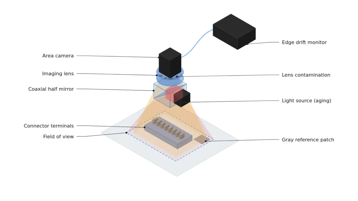
② Optical setup	Illumination	Coaxial illumination, matte gray reference patch in the FOV corner	For highly reflective metal terminals. Patch dedicated to luminance drift
② Optical setup	Sensor & lens	2448 × 2048 px (pixel pitch 3.45 µm), focal length 25 mm	Design assumption. Magnification 0.230× (calculated)
② Optical setup	WD (working distance)	120 mm or more must be secured	Thin-lens approximation object distance about 134 mm (calculated). Measure including coaxial light housing
② Optical setup	FOV & pixel resolution	FOV 36.7 mm × 30.7 mm, 15 µm/px	2448 px × 15 µm = 36.72 mm (calculated)
③ Algorithm	Mean luminance (reference patch 64 × 64 px)	Warning −5%, stop −10%	Metric dedicated to illumination degradation. Reference is the mean over stable operation
③ Algorithm	Sharpness (Laplacian variance, 1/4 downscale)	Warning −15%, stop −30%	Computed on 612 × 512 px. Metric for lens contamination and focus drift
③ Algorithm	Embedding distance (Mahalanobis)	Warning > p99, stop > p99.9 for 20 consecutive frames	Based on the feature distribution of 500 good-part images. Reuses backbone features
③ Algorithm	Smoothing	EWMA λ = 0.05	Equivalent to a 2 ÷ λ − 1 = 39-frame moving average

Table implication. The 45 µm scratch in ① is exactly 3.0 px at the 15 µm/px of ②, so widening the blur by just 1 px (15 µm) can push it below the detection floor. For that reason, the sharpness stop threshold of −30% in ③ may look reasonable statistically but can be too loose for a 3 px defect, and it is likely to need tightening to within the measured sharpness drop that corresponds to 1 px of blur. Drift thresholds must be back-calculated not only from statistics but from the px occupancy margin of the minimum defect.

5. When the Opposite Approach Wins

• Processes with a high defect rate where labels accumulate quickly: If re-inspection results come back at tens of cases or more every hour, tracking output accuracy directly becomes the more accurate form of monitoring.
• High-mix lines where product types change frequently: The embedding reference distribution changes with every changeover, so if per-type references are hard to maintain, running only reference patch luminance and sharpness is more realistic.
• Equipment where periodic calibration is enforced at short intervals: If the calibration interval is sufficiently shorter than the drift rate, the benefit of continuous monitoring is small.

On highly reflective metal terminals, diffuse reflection components and surface finish variation can shake the sharpness metric itself, so the thresholds above cannot be confirmed before sample testing.

Field Note

In terminal inspection on a high-speed assembly line, over-detection once crept up little by little over several weeks. I first considered retraining the model, but when I traced the sharpness metric back through the stored images, it had already been declining gently from about two weeks before the over-detection increased. The cause was a fine oil film on the front of the lens. After that, placing a gray reference patch in the corner of the FOV and monitoring luminance and sharpness with an EWMA let us bring the cleaning schedule forward. Still, I believe the thresholds have to be set again by measurement for each piece of equipment.

Field Checkpoints

• Is a WD of 120 mm or more secured by measurement — verify including the coaxial light housing and the reference patch bracket.
• Has the surface material and reflectance of the target been identified first — check how much the finish variation of the metal terminal shakes the sharpness metric.
• Is luminance drift measured on a fixed reference patch inside the FOV rather than on the product area.
• Were the reference values of the three metrics set from good-part statistics over a period of stable operation rather than right after installation.
• Are the warning and stop thresholds separated, and is a stop linked to a decision hold and re-inspection flag.
• Is it recorded whether the metrics return to their reference values after lens cleaning or illumination replacement.