Must Every Normal Patch Be Remembered? — Edge Deployment and Coreset Design for Memory-Bank Anomaly Detection

EDGE AI / ALGORITHM

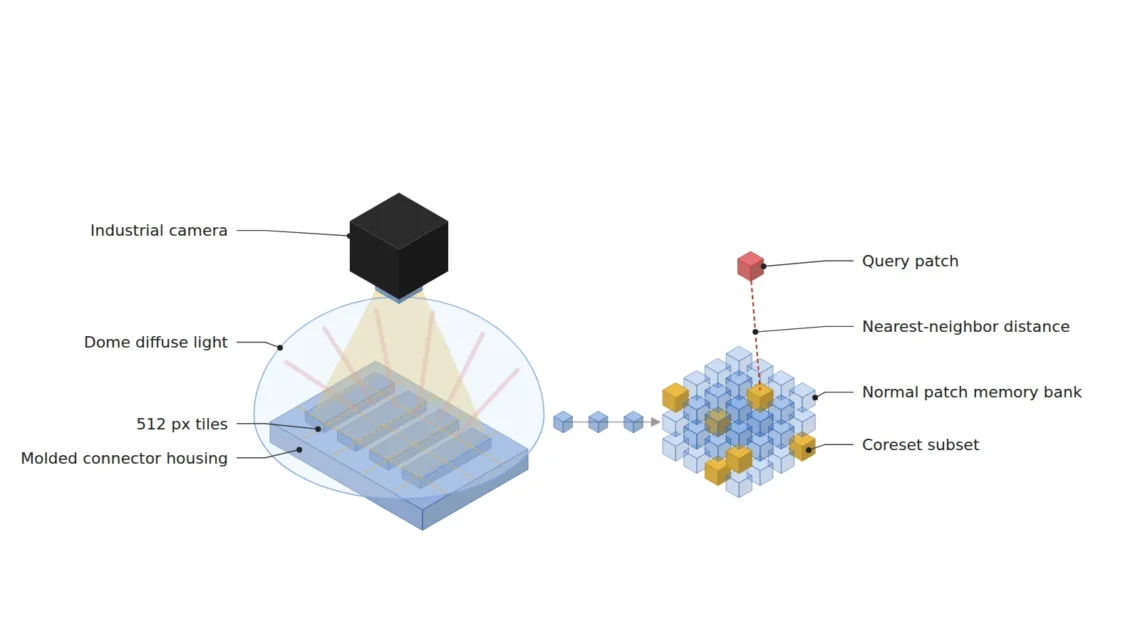
In processes where defect samples are hard to collect, such as injection-molded connector housings, memory-bank-based anomaly detection (the PatchCore family), which learns from good parts only, is often chosen. Patch features of good images are extracted from a pretrained backbone and stored, and each patch of an inspection image is given an anomaly score by how far it is from the nearest good patch. This structure, which ran well on a server, reveals two problems at once — memory and search latency — the moment it is moved to an edge device.

Left unaddressed, the cost comes out in two directions. Shrink the memory bank without grounds, and part of the normal variation drops out of memory, increasing overkill where good parts are judged anomalous; do not shrink it, and nearest-neighbor search latency exceeds the line takt, so full inspection retreats to sampling inspection. The moment the threshold is raised to reduce overkill, small dark specks quietly start to pass. Either way, the advantage of the “knowing only good parts is enough” approach disappears on the floor.

The solution is to treat the memory bank not as model weights but as a designable data structure. First fix the minimum defect size from the input resolution and patch size, calculate the raw memory bank size under that condition, and then choose the coreset subsampling ratio on the trade-off among memory, search latency and detection performance. This article does not cite paper figures; it follows the calculation using principles and design assumptions only.

The detection floor of memory-bank anomaly detection is set not by the model but by the µm that one patch cell covers.

1. Input Resolution and Patch Size Set the Minimum Defect Size

Point. In the memory-bank approach, the minimum detectable defect size is determined by the input resolution and the backbone’s feature stride before the amount of training data.

Reason. The anomaly score is computed per patch feature. If the stride of the backbone’s intermediate layer is 8, one feature map cell summarizes an 8 × 8 px input area, and adding 3 × 3 neighborhood aggregation makes the area actually reflected even wider. The smaller the share of that area a defect occupies, the more the patch feature is pulled toward normal texture and the lower the anomaly score. The more decisive step is the preprocessing that shrinks the camera original to the backbone input size. Pixel resolution coarsens by the downscale factor, and at that moment a small defect loses its presence within the patch.

Example. Imaging an FOV of 49 mm × 41 mm with a 2448 × 2048 px camera gives a pixel resolution of 20 µm/px. Shrinking this whole image to 512 × 512 px makes it about 95.7 µm/px horizontally, so an 80 µm diameter dark speck does not even reach 1 px. Conversely, cutting it into 20 tiles of 512 px (5 × 4, with partial horizontal overlap) to keep the original resolution makes the same speck 4 px, occupying half the width of a stride 8 patch cell (160 µm).

Point. The first calculation in minimum defect design is µm/px × stride = patch cell size (µm). Only after tiling and FOV are set so that the defect occupies around half the cell width can the memory bank size be discussed.

2. Raw Memory Bank Size and Coreset Subsampling

Point. Storing every good patch as the principle dictates easily makes the memory bank exceed an edge device’s memory, so coreset subsampling is not an option but a premise.

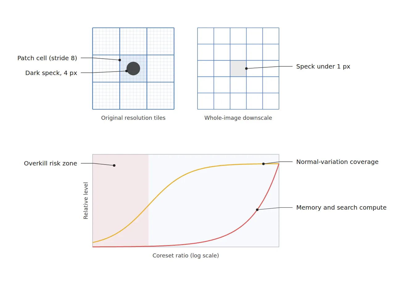
Reason. Memory bank size is the number of good images × tiles per image × patches per tile × feature dimension × data type size. Because it is a product, the moment tiles are added to preserve resolution, memory grows in direct proportion. Coreset subsampling is a greedy selection procedure (greedy coreset) that keeps only representative patches evenly covering the feature space, and unlike random sampling it tends to preserve rarely occurring normal variation first. Even so, the lower the ratio, the less rare variation is preserved.

Example. With the design assumptions of 100 good images, 20 tiles per image, 64 × 64 = 4,096 patches per tile, feature dimension 384 and FP16 (2 byte), the raw memory bank is 8,192,000 patches × 768 byte ≈ 6.29 GB. Reducing it with a 1% coreset gives 81,920 patches, about 62.9 MB, which fits into an edge device’s memory budget. Reducing further to 0.1% gives about 6.3 MB, but the risk grows correspondingly that rare normal variation — gloss changes around gate marks, mold parting lines, subtle color shifts between lots — drops out of the bank.

Point. The coreset ratio is not a value back-calculated from a memory target but one decided after confirming, with a good-part validation set, which normal variation can be dropped from memory.

3. Nearest-Neighbor Search Latency — Where the Edge Hits the Wall First

Point. In edge deployment, what reaches its limit first is usually not memory but the compute of nearest-neighbor search.

Reason. If every patch of an inspection image computes distances to the entire memory bank, compute is proportional to query patch count × bank size × feature dimension. Cutting the coreset ratio tenfold cuts memory and exhaustive search compute tenfold together — a linear relationship. Approximate nearest-neighbor search (index partitioning, vector quantization) greatly reduces this compute, but at the price that approximation error mixes into the anomaly score itself. Because the anomaly score is “the distance to the nearest good patch”, when approximate search picks a slightly farther neighbor, the scores of good patches rise systematically and lean toward overkill.

Example. Under the assumptions above, one image has 20 × 4,096 = 81,920 query patches. An exhaustive search against a 1% coreset bank (81,920 patches) requires 81,920 × 81,920 × 384 ≈ 2.58 × 10¹² multiply-accumulates, which is very heavy relative to an edge compute budget. With a 0.1% bank it drops tenfold to about 2.58 × 10¹¹. So the practical order is to lower the coreset ratio first as far as validation allows, fill only the remaining shortfall with approximate search, and always compare the shift in the good-part validation set’s score distribution before and after applying the approximation.

Point. Trying to solve search latency only with a faster device keeps raising the cost. First see the structure in which query count (tiling) and bank size (coreset) multiply to create latency.

A single coreset ratio moves memory and search compute together by the same factor.

4. Core Framework — Matching Table

Category	Item	Specification / Parameter	Basis · Notes
① Minimum defect size	Dark speck · foreign particle	Diameter 80 µm or more	Design assumption. 4 px at 20 µm/px, half a patch cell width
① Minimum defect size	Flow mark · scratch	Width 60 µm, length 400 µm or more	Design assumption. Width 3 px, length 20 px
① Minimum defect size	Short shot (incomplete fill)	Width 200 µm or more	Design assumption. 10 px, 1.25 patch cells
② Optical setup	Illumination	Dome diffuse illumination	For matte PBT surfaces. Glossy gate areas cannot be confirmed before sample testing
② Optical setup	Camera	2448 × 2048 px, 3.45 µm pixel	Design assumption. Sensor width approx. 8.45 mm
② Optical setup	Lens	Focal length 25 mm, magnification approx. 0.17×	Calculated: 8.45 mm ÷ 49 mm
② Optical setup	WD (working distance)	150 mm or more must be secured	Calculated object distance approx. 170 mm (from principal plane). Measure including dome light height
② Optical setup	FOV · pixel resolution	FOV 49 mm × 41 mm, 20 µm/px	Calculated: 49,000 µm ÷ 2,448 px ≈ 20.0 µm/px
③ Algorithm	Input tiling	20 tiles of 512 × 512 px (5 × 4), no downscaling	Whole-image downscaling gives 95.7 µm/px, speck under 1 px
③ Algorithm	Patch features	Stride 8 layer, 3 × 3 neighborhood aggregation, dimension 384, FP16	Calculated patch cell 160 µm (20 µm/px × 8)
③ Algorithm	Memory bank · coreset	Raw 8,192,000 patches (≈ 6.29 GB) → 1% coreset 81,920 patches (≈ 62.9 MB)	Design assumption for 100 good images. Decide on 0.1% after validation
③ Algorithm	Decision	k = 1 nearest distance, threshold = 99.9th percentile of good validation set scores	Design assumption. Re-estimate threshold when approximate search is applied

Table takeaway. In a 160 µm cell from 20 µm/px × stride 8, an 80 µm speck is 4 px, half the cell width, barely meeting the detection premise, and shrinking the whole original to 512 px gives 95.7 µm/px, making it vanish in principle regardless of memory bank size. In other words, 20 tiles are the price of resolution, and that factor of 20 multiplies both the raw memory bank size and the query count at the same time, so that even with a 1% coreset about 2.58 × 10¹² multiply-accumulates per image remain — this is the real bottleneck of the design.

5. When the Opposite Approach Wins

• When enough defect samples can be collected and defect types are fixed: A supervised segmentation or classification model is favorable in both boundary precision and inference cost. Nearest-neighbor search itself is unnecessary.
• Products with very large normal appearance variation: With many color variants or large texture differences between lots, the memory bank grows sharply or overkill increases. Consider separate banks per variant or a different method first.
• When the inspection area is very small: If the ROI is only a few mm, the raw bank is small and exhaustive search without a coreset may fit within the takt. In that case subsampling is rather an unnecessary loss of information.

Among molded parts, glossy surfaces and transparent resins have their patch features shaken strongly by diffuse and specular reflection, changing the width of normal variation itself, so the required bank size and coreset ratio cannot be confirmed before sample testing.

Field Note

In injection-molded connector housing inspection, when I reduced the coreset ratio from 1% to 0.1%, memory and search time dropped to about one tenth as calculated, but I saw glossy patches around the mold gate drop out of the bank, with overkill concentrating only at that location. Looking at the overall overkill rate alone, the cause was not visible; the structure became clear only after mapping which tile and which coordinates the overkill concentrated in. In the end I compromised by keeping a higher ratio only for tiles around the gate, but I think whether this allocation fits other molds has to be checked again with samples.

Field Checkpoints

• Is a WD of 150 mm or more secured by measurement — verify including the dome light height and the position of the camera viewing port.
• Has the surface material and reflectance of the target been identified first — separate matte areas from glossy gate areas and look at the width of normal variation for each.
• Has the patch cell size been calculated as µm/px × stride, and does the minimum defect occupy around half the cell width.
• Do the raw memory bank size (images × tiles × patches × dimension × byte) and the post-coreset size fit within the device’s memory headroom.
• Does the search compute per image (query count × bank size × dimension) fit within the line takt.
• Have the score distribution of the good validation set and the overkill location map been compared before and after applying the coreset and approximate search.