AOI Only Says “Defective” — How Vision Language Models Fill the Gap in Judgment Rationale

EDGE-AI · ALGORITHM

An AOI (Automated Optical Inspection) unit just flagged one PCB as defective. The screen shows the coordinates, a cropped image, and an anomaly score of 0.87. But that is not what the line actually needs. Whether the next step is a solder-bridge rework, a re-mount, a simple wipe, or a process-parameter correction depends entirely on what kind of defect it is.

Leaving this gap unaddressed carries two costs. One is re-inspection labor: with no judgment rationale, a person has to re-verify everything, and the moment they do, the labor savings from automated inspection evaporate. The other is a more subtle cost — you cannot tabulate occurrence trends by defect type, so the feedback loop for process improvement breaks down. The line keeps inspecting, but the yield never improves, because that is exactly the condition this creates.

The fix is not to make the detector more accurate — it is to add a layer that attaches meaning after detection. A Vision Language Model (VLM) defect classifier maps images and natural language into the same representation space, so it can output, in words, why a given cropped region is being read as defective.

An inspection system’s value is no longer decided by how many defects it catches, but by whether it can say what it caught.

The interpretability gap is a structural problem, not a performance problem

Point. The black-box nature of conventional AOI is not the kind of problem you solve by swapping the model.

Reason. CNN-based anomaly detectors are designed to output a distance from the normal distribution. There is no axis in the output space for “defect type,” so no matter how much you refine the model, type information never comes out of it. You can attach type labels and retrain as multi-class classification, but that path demands labeled data for dozens of images per type, repeated every time a new defect type appears.

Example. VLM research published in 2026 across industrial-defect domains commonly starts from this exact point. Conventional AOI performs well at anomaly detection, but lacks the semantic interpretability needed to classify what it detected. In the same body of work, a single multimodal model trained on mixed-product data was shown, in one case study, to be able to distinguish defects across different products from natural-language prompts alone.

Point. In other words, Vision Language Model defect classification is not a replacement for the detector — it is a complementary layer sitting on a different output space.

Evidence selection — don’t judge from a single frame

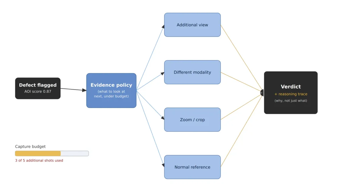
Point. In the 2026 research stream, the most practical piece is not the judgment itself but the policy that decides what additional evidence to gather.

Reason. A human inspector, on encountering an ambiguous crop, naturally tilts the angle to look again, zooms in, or lines the case up against similar normal-part examples. A fixed pipeline cannot do any of that — it judges from the first frame’s information alone. The result is that both false positives and false negatives spike in exactly the ambiguous boundary cases.

Example. The ActiveInspect research published in 2026 formalizes inspection as a sequential evidence-selection problem under a budget constraint. The policy itself decides whether to request an additional shot, try a different modality, expand the candidate region, retrieve a matching normal-part reference, or terminate the judgment here. From an inspection-hardware standpoint, this means the model decides which of two lighting angles to shoot as the extra frame, so the shot-count budget directly becomes the tact-time budget.

Point. This is where optical setup matters again. The kind of evidence a model can choose to request is limited to only what the hardware has already prepared in advance.

Small-label systems — a realistic path to adoption

Point. The practical advantage of adopting a VLM is not inference cost — it is label acquisition volume.

Reason. Gathering dozens of images per defect type to build a new line takes months. And the line is already running during that interval, so whether labeling can start from a near-zero sample count decides whether adoption is even feasible.

Example. A 2026 study on VLM adaptation for small-sample targets reported a case in which, using only 9 training instances from a dominant tile-family category, it reached a maximum mAP@50 of 64.9%. That figure should not be read as a production go/no-go threshold, but rather as a starting point sufficient for a human not to have to fully hand-label early-stage type classification. This presumes an operating model where, for the first several weeks, human-inspector confirmations are recovered as labels and the system is incrementally improved.

Point. So the number that matters when budgeting isn’t target accuracy alone — it’s three figures: starting accuracy / label-recovery rate / time to target.

A VLM is not a technology that replaces the inspector — it is a technology that turns the inspector’s judgment into data.

Core framework — minimum defect size / optical setup / algorithm parameter matching table

Category	Item	Spec / Parameter	Rationale · Notes
① Minimum defect size	Solder bridge	Min. width 80 µm	Shape must be resolved for type classification
① Minimum defect size	Part misalignment / lift	Position offset 150 µm	Relative-to-reference judgment
① Minimum defect size	Surface contamination	Min. diameter 60 µm	Detection by AOI, type classification by VLM
② Optical setup	Camera	12 MP color, 2/3-inch	Reserves resolution margin for the post-crop VLM input
② Optical setup	Lens	Focal length 50 mm, F/5.6, 8 µm/px	An 80 µm bridge resolves to 10 px
② Optical setup	WD (working distance)	150 mm or greater — mandatory	Verified by measurement to avoid interference between multi-angle lighting rings
② Optical setup	Lighting	Coaxial + 2-tier low-angle ring, independently addressable per segment	Pre-arranges, in hardware, the range of views the evidence-selection policy can choose from
② Optical setup	Illuminance	Per-channel uniformity within ±5%	Brightness offset between channels leaks into type misclassification
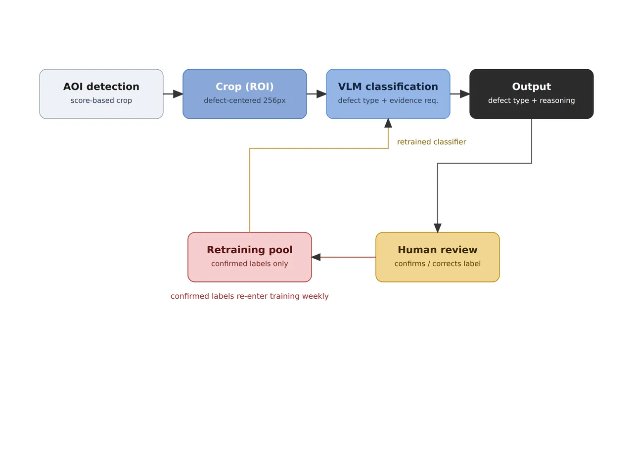
③ Algorithm	Pipeline	AOI detection → crop → VLM type classification and rationale generation	The VLM is not a substitute for detection
③ Algorithm	Input crop	256 × 256 px centered on the defect + 1 normal-reference frame	The paired reference input contributes to classification stability
③ Algorithm	Evidence budget	Up to 2 additional shots per unit	Counted directly against the tact-time budget
③ Algorithm	Confidence gate	Classification confidence below 0.6 routes to human confirmation	Mandatory for early-stage operation
③ Algorithm	Label recovery	Human-confirmation results feed the full retraining pool	Weekly retraining cadence

Table takeaway. The 2-tier independently addressable lighting in ② and the 2-shot evidence budget in ③ are a matched pair by design. With only a single lighting channel, the evidence-selection policy has no choice but to expand the candidate region, and most of the benefit of an ActiveInspect-style approach is lost. This is exactly why the optical setup has to be reopened at the point you decide to adopt the algorithm.

Related Patents (Confirmed to Exist)

Patent No.	Title	Assignee
US 10,599,951 B2	Training a neural network for defect detection in low resolution images	KLA-Tencor Corporation
US 2022/0222806 A1	Machine learning-based classification of defects in a semiconductor specimen	Applied Materials Israel Ltd.

Patents whose assignee could not be explicitly confirmed were excluded from citation.

Conditions Favoring the Opposite Approach

• Lines where defect types are fixed at 2–3 categories and new types almost never appear: with per-type labels already well gathered, a conventional multi-class CNN is favorable on both inference cost and latency.
• High-speed lines where tact time runs in tens of milliseconds: VLM inference latency becomes the bottleneck, so a practical setup is to split type classification off into an offline batch.
• Fully unmanned lines where the judgment rationale does not need to be read by a person: the value of interpretability drops.

Model performance is heavily skewed by product and defect distribution, so it cannot be generalized before sample testing.

Field Checkpoints

• Is 150 mm or more of WD actually confirmed by measurement — check it with both lighting tiers mounted at once.
• Does the lighting and shot-angle channel count that the evidence-selection policy can choose from actually exist in the hardware.
• Are all three figures — starting accuracy / label-recovery rate / time to target — written into the budget.
• Are the input and response-time budgets for the human-confirmation queue defined for confidence-gate cases below the threshold.
• Is a path built for human-confirmation results to automatically feed the retraining pool — without it, starting accuracy simply stays the final accuracy.