Can Five Defect Samples Stand Up a Few-Shot Anomaly Detection Line?

ALGORITHM

Catching all five defects still leaves recall possibly as low as 55 %, and claiming 95 % takes 59.

Taking a molding line with only a handful of defect samples, I calculated what few-shot anomaly detection can set up, what it cannot prove, and what the threshold and lighting have to carry.

About 11 min read

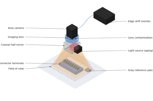
The surface of a matte injection-molded housing has a fine texture that scatters light in every direction, a diffuse reflection¹ surface. A 50 μm wide scratch on it sinks into the texture under frontal light and only rises as a bright line under dark-field illumination², which skims light across at a low angle. The trouble is that such defects are rare early in production. With thousands of good-part images piling up a day and only five defects, anomaly detection³, which finds defects by how far they stray from normal, comes up as the alternative.

The question is simple: can an inspection line be built on five defect samples? I answer it in two parts: setting up the detection criterion, and proving how many defects that criterion misses. The first can start with five, but the calculation says the second does not end with five.

The “few” counts normal images

In few-shot⁴ industrial anomaly detection research, the “few” usually refers to the number of normal images. FastRef (arXiv 2506.21398, posted June 26, 2025), presented as a CVPR 2026 poster, refines the prototypes⁵ that represent normal features when only 1, 2 or 4 normal images are given, and is evaluated on the MVTec, ViSA, MPDD and RealIAD datasets. It alternates a stage that updates the prototypes with a stage that suppresses anomalous components, and is built to be added on top of existing methods such as PatchCore.

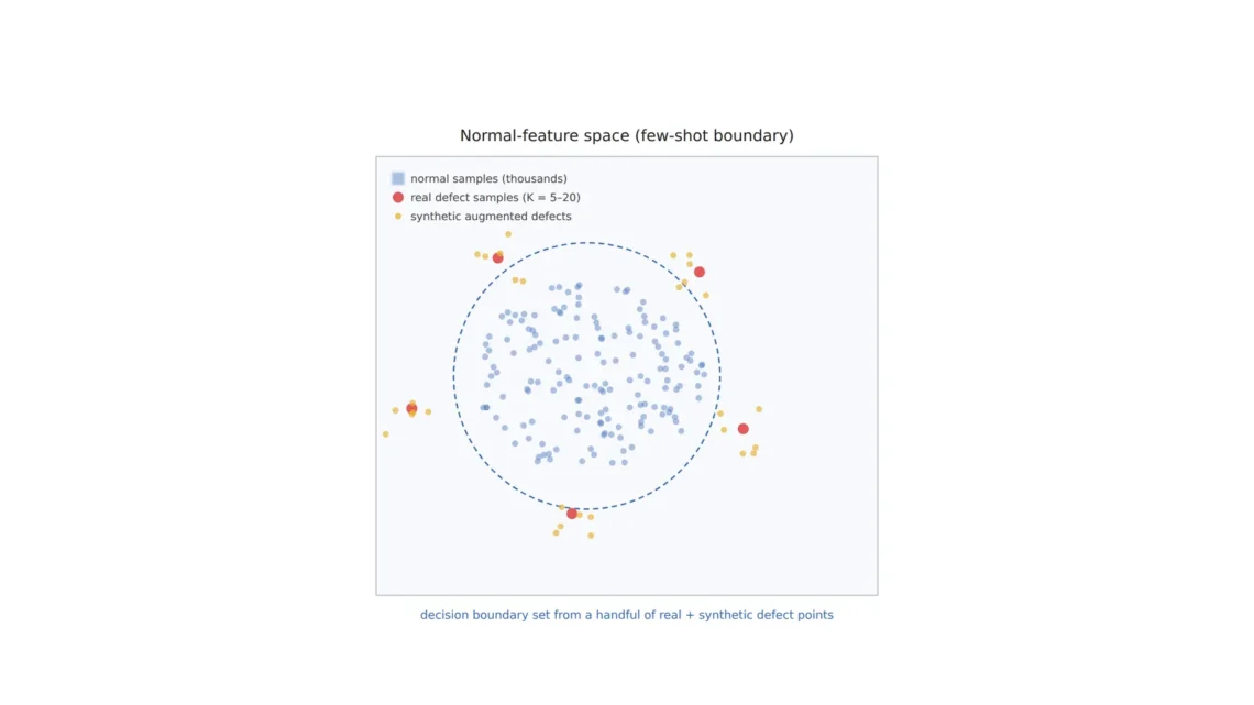
In this setting only normal images go into training, because the model learns what normal looks like and scores how far each image strays from it. Five defect images are therefore closer to validation material than to training material. I see this distinction as the first thing to settle when putting few-shot anomaly detection on a line. If the five are validation material, the next question is what those five can prove.

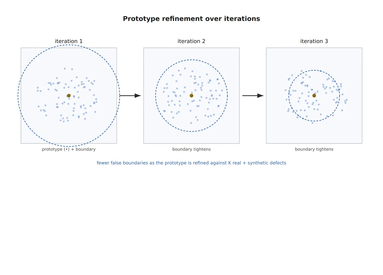
The prototype centers in the figure stand for where normal features gather, and points outside the boundary are judged anomalous. Normal data decides where the boundary is drawn, and only defect data can say how many real defects that boundary catches. The two questions need very different amounts of data, and that difference is where the problem starts.

Catching all five still allows recall as low as 55 %

Suppose the model catches all five defects. It is tempting to write recall⁶ as 100 %, but five images are far too few to support that number. If the true recall is r, the chance of catching all five is r⁵, and the r at which that chance falls to 5 % is 0.05^(1/5) = 0.549. At 95 % confidence, all that catching all five says is that recall is at least 55 %. That value is the lower confidence bound⁷ on recall.

Working backward gives the number needed. Claiming recall of 95 % or more at 95 % confidence with zero misses takes ln 0.05 ÷ ln 0.95 = 58.4, so 59 defects. For 90 % it takes 29, and for 99 % it takes 299. Gathering 59 real defects early in production is hard. So I treat the first months as a period when the proof is unfinished, and keep something like sampled visual inspection alongside to catch the defects the model misses.

Thousands of normal images set the threshold

While proof on the defect side lags, the normal side has numbers to spare. If the anomaly score⁸ threshold is set from the distribution of normal scores, the false calls⁹ it produces can be measured with normal images alone. Assuming normal scores follow a normal distribution, a threshold at mean + 2σ flags 2.28 % of good parts, which on a line inspecting 3,000 parts an hour sends 68 an hour to re-inspection. Raising it to mean + 3σ gives 0.135 %, or 4 an hour.

The normal-distribution assumption often fails in the tails, so it has to be checked on real normal images. Claiming a false-call rate of 0.135 % or less at 95 % confidence with zero false calls takes about 2,200 normal images, an amount a production line gathers within a day. I fit the threshold to the score distribution of thousands of normal images, never to the five defects. The five are used only to check that all of them land above that threshold.

What synthetic defects can and cannot do

With defects scarce, making some is a natural thought. KLA’s US patent US10599951B2 (priority date March 28, 2018; granted March 24, 2020) describes a setup in which a neural network handling high-resolution images synthesizes defect images to build a training set, and a low-resolution inspection network trained on that set then finds defects on other specimens. The idea is to fill training material with synthetic defects¹⁰ where real defects are hard to gather in quantity.

Synthetic defects are very useful for training and tuning. They show ahead of time whether the score reacts to a synthetic scratch and which shapes sit on the boundary near the threshold. They cannot be counted toward proving recall, though. A synthetic defect is a defect we imagined, with no guarantee that it represents the shape of a defect appearing on the real line for the first time. Adding 40 synthetic images to 5 real ones leaves the count usable for proof at 5.

Synthetic defects are practice problems. Real ones are the exam. Only the exam can be graded.

Lighting sets the width of the normal distribution

If the threshold comes from the normal score distribution, narrowing that distribution is the same as raising detection power. The texture of a matte molded surface shifts a little from lot to lot, and as it shifts the features of normal images wobble and the standard deviation of normal scores grows. Keep the threshold at mean + 3σ of the old distribution while lot texture grows the standard deviation 1.5 times, and the false-call rate goes from 0.135 % to 2.28 %, about 17 times as many. Raise the threshold again and false calls fall, but now faint scratches drop below it.

Dark-field lighting works toward narrowing that width. Under low-angle light the flat texture sinks dark and only the edges of a scratch send light back toward the lens, so texture changes weigh less on the features and the scratch stands out more. However good prototype refinement is, if the contrast between texture and scratch in the raw image is small, there is no material to separate the overlapping score distributions. How much texture roughness and gloss vary by lot, and so how much the normal distribution widens, cannot be guaranteed before a sample test.

When supervised learning wins on a 50 μm scratch line

Before standing up the line, decide three things in the same table: how many pixels the scratch occupies, how much the lighting narrows the normal distribution, and how the threshold and validation count are set. Taking 16.7 μm per pixel so a 50 μm scratch spans 3 px, a 2,448 × 2,048 px sensor with 3.45 μm pixels gives a field of view of 40.8 × 34.1 mm at a magnification of 0.207×. A 25 mm lens puts the housing about 146 mm from the principal plane of the lens by the thin-lens approximation, and since the dark-field ring light sits low and close to the part, the clearance between lens and ring has to be checked as the actual WD¹¹.

Item	① Minimum defect size	② Optical setup · lighting · WD	③ Algorithm parameters
Resolving the scratch	50 μm wide = 3 px (16.7 μm/px)	2,448 × 2,048 px, 3.45 μm pixels, 0.207× magnification, field of view 40.8 × 34.1 mm. 25 mm lens, object distance about 146 mm (thin-lens approximation; check WD from the lens front on the datasheet)	Build prototypes from normal images (the few-shot setting starts from 1 to 4 normal images); patch-level anomaly scores
Lighting · normal distribution	Contrast between texture and scratch	Low-angle dark-field ring light; check the WD left after the ring height. Collect samples of texture change by lot	Log the normal-score standard deviation per lot. If it grows 1.5×, false calls at a 3σ threshold go from 0.135 % to 2.28 %
Threshold · validation	5 defects = recall lower bound 55 %	At least 2,200 normal images with the same lens, WD and lighting	Set the threshold from the normal distribution (mean + 3σ, about 4 false calls per hour). Proving 95 % recall takes 59 real defects (synthetic excluded)

With all three rows filled, inspection can start on five defects, and what remains unproven gets written down as well. Lighting and thousands of normal images set the normal distribution, and the proof on the defect side stays open until real defects reach 59.

There are also places where supervised learning fits better than few-shot anomaly detection. If normal appearance itself swings widely from lot to lot with no way to narrow the normal distribution, or if defect types are fixed and hundreds of each are already on hand, training a classifier on labels per defect type makes the threshold easier to handle. Which side does better on a real line depends on material and process variation, so it cannot be guaranteed before a sample test.

Turning a defect-sample count into a lower confidence bound is the first number an engineer planning inspection for a new line needs, and on the quality assurance side it becomes the basis for shipping decisions. When bringing in an anomaly detection model, ask first how many real defects stand behind its accuracy figure. This article explains technology and is not investment advice. See our Disclaimer.

Field Note

If a new line were starting on five defect samples, my first step would be a table of which defect types those five represent. Next would come a score distribution from 2,200 or more normal images, a measurement of false calls at a mean + 3σ threshold, and a check that all five defects land above it. Until real defects reach 59, sampled visual inspection would run alongside to catch what the model misses, with a row added to the table for each new defect type.

Field Checkpoints

Once the normal score distribution and the defect check are in, use the items below to judge whether few-shot anomaly detection should inform production decisions.

• WD: with the 25 mm lens, does the actual WD from the front of the lens to the housing leave room for the low-angle ring light? (thin-lens object distance about 146 mm)
• Was the threshold set from the score distribution of 2,200 or more normal images?
• Is recall on the five defects written as its lower confidence bound (55 %) in place of 100 %?
• Is another inspection in place to catch misses until real defects reach 59?
• Are synthetic defects left out of the count used to prove recall?
• Is the normal-score standard deviation logged per lot, with lighting and threshold reviewed when it grows 1.5 times or more?
• Has the contrast between texture and scratch under dark-field lighting been checked on samples?

Frequently Asked Questions

Can anomaly detection start with no defects at all?

A criterion can be set up from normal images alone. The few-shot setting is being studied to work with as few as one to four normal images, and defect images do not go into training. With zero defects, though, there is no way to confirm the score even reacts to real defects, so I would first check the response with synthetic defects and add real defects to the validation count as they appear.

How do I choose between mean + 2σ and 3σ?

By the ratio between the cost of a false call and the cost of a miss, and by where faint defects score. On a 3,000 parts-per-hour line, 2σ creates 68 re-inspections an hour and 3σ creates 4. If defect scores sit well above the 3σ threshold, 3σ is cheaper; if faint defects bunch between 2σ and 3σ, lowering the threshold and accepting the re-inspections is right.

When should the model be retrained?

When normal appearance changes and when a new defect type is confirmed. If the mean and standard deviation of normal scores move after mold maintenance or a change of resin lot, rebuild the prototypes from new normal images and set the threshold again from the new distribution.

Glossary

• [1] Diffuse reflection diffuse reflection
  Reflection that scatters light in many directions from a rough surface. It is strong on matte molded surfaces. ↩
• [2] Dark-field illumination dark-field lighting
  Lighting at a low angle that makes flat surfaces look dark and scratch edges look bright. ↩
• [3] Anomaly detection anomaly detection
  Finding anomalies by how far they depart from a learned picture of normal. Defect types need not be defined in advance. ↩
• [4] Few-shot few-shot
  A setting meant to work from very few training images. In industrial anomaly detection it usually means 1 to 4 normal images. ↩
• [5] Prototype prototype
  Reference points that represent normal features. A new image is scored by how far its features lie from them. ↩
• [6] Recall recall, sensitivity
  The share of real defects that the inspection catches as defects. ↩
• [7] Lower confidence bound lower confidence bound
  The bound below which the true value is unlikely given the observations, at a set probability (5 % in the text). ↩
• [8] Anomaly score anomaly score
  A number for how far an image or patch departs from normal. Crossing the threshold means a defect call. ↩
• [9] False call false positive
  The mistake of calling a good part bad. It costs re-inspection labor and time. ↩
• [10] Synthetic defect synthetic defect
  A defect image made by image processing or a generative model in place of a real one. It is used for training and kept out of recall proof. ↩
• [11] WD working distance
  The distance from the front of the lens to the inspected part. It decides how much room fixtures like a ring light have in between. ↩

References

• Long Tian et al., “FastRef: Fast Prototype Refinement for Few-Shot Industrial Anomaly Detection”, arXiv:2506.21398, 2025-06-26. arXiv
• CVPR 2026 poster, “FastRef: Fast Prototype Refinement for Few-shot Industrial Anomaly Detection”, session of 2026-06-07. cvpr.thecvf.com
• KLA-Tencor Corp., US10599951B2 “Training a neural network for defect detection in low resolution images”, priority date 2018-03-28, granted 2020-03-24. Google Patents

Related reading — Does Memory-Bank Anomaly Detection Need to Remember Every Normal Patch? · Overdetection or Missed Detection, Which One Costs More? · Deep Learning vs. Rule-Based Algorithms, When to Use Which