Why Does a Lightweight Model Lose the Finest Defects First? — Designing Edge Segmentation with Knowledge Distillation

EDGE AI / ALGORITHM

In PCB trace appearance inspection, a server-class segmentation model paints the boundary of a trace nick as narrow as 30 µm accurately along its edge. But when the same model is to be placed on an edge device next to the line, its compute and memory exceed the allowed range several times over. So a lightweight model with fewer channels is trained from scratch, and a phenomenon appears in which the overall average metric barely drops, yet only the boundary of the finest defect is smeared or disappears altogether.

If the model is deployed by looking only at the average metric, the cost arises at the smallest defect. A nick 3 px wide is such a tiny fraction of all pixels that it hardly moves the average mIoU. The dashboard looks normal while precursors of trace opens ship as they are, and when they surface late in electrical test or in the customer’s process, rework and return costs come back several times over. A paradox also arises in which the record of having passed inspection actually delays root-cause tracing.

The solution splits into two layers. First, distill the probability distribution the teacher model produces near boundaries (soft labels) and its intermediate feature maps into the student model — knowledge distillation — so that the boundary information itself is transferred. Second, block in advance, at the architecture design and optical setup stage, the region that distillation cannot restore — the zone where the student model’s output resolution becomes coarser than the defect width. Distillation is only a tool for moving information; it cannot newly create contrast that the optics failed to create.

What distillation transfers is not the answer but how much the teacher hesitated at the boundary.

1. Soft Labels Carry the “Width” of a Boundary

Point. The core value of knowledge distillation lies not in copying the teacher’s answer but in conveying to the student how confident the teacher is at boundary pixels.

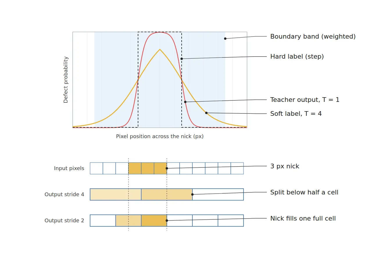
Reason. A human-made hard label splits defect and background into a step of 0 and 1. In a real image, however, a defect boundary is recorded as a gradual brightness transition spanning 2 to 3 px because of the lens point spread (PSF) and the illumination angle. The teacher model outputs intermediate probabilities such as 0.3 and 0.6 in this transition zone. Dividing the logits by a temperature parameter T before the softmax (softmax(z/T)) flattens the distribution, and the differences among these intermediate probabilities turn into gradients large enough for the student to learn from. At T = 1, the probability of pixels just slightly off the boundary sticks to 0 or 1 and the information disappears; if T is too large, even the distinction between defect and background blurs.

Example. At a pixel resolution of 10 µm/px, a 30 µm trace nick is 3 px wide. Trained with hard labels alone, a lightweight model tends to be confident only about the center 1 px of those 3 px and hands both sides over to the background. With the design assumption T = 4 and the loss L = 0.5 · CE(hard) + 0.5 · T² · KL(soft), the intermediate probabilities at boundary pixels are reflected directly in the loss, easing the effect in which the nick width shrinks to 1 px. The T² factor is a conventional term that compensates for the gradient magnitude reduced by the temperature.

Point. Temperature is not about “how soft to make it” but a parameter that decides how many px of the boundary transition zone are used as the learning signal. Only when the defect width and the PSF width are known first can the range for sweeping T be set.

2. Feature Map Distillation — Transferring the Representation Before the Output

Point. If only the output probabilities are distilled, the student learns “what to paint” but not “what to look at when painting”.

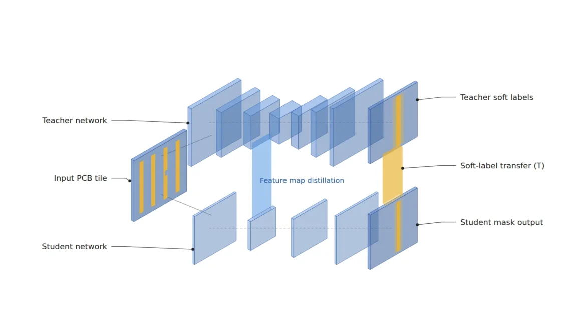
Reason. A lightweight model has few channels and cannot sufficiently preserve high-frequency edge information in its early layers. The soft labels at the output are already the compressed result of many layers, so their signal is too weak to revive the fine edge representation lost in the intermediate layers. Feature map distillation matches the channel count of the teacher’s and student’s intermediate feature maps with a 1 × 1 convolution adapter, then adds the difference between the two feature maps (MSE) to the loss. Which layer is chosen here is decisive. If a deep layer with too low a spatial resolution is chosen, a 3 px wide defect has already melted into a single cell and there is no information left to transfer.

Example. For a 512 × 512 px tile input, the feature map of a stride 8 layer is 64 × 64 cells, and one cell represents 8 px, that is, an 80 µm area. A 30 µm nick falls short of half the cell width but is large enough to clearly change the cell’s feature value. In a stride 32 layer, by contrast, one cell is 320 µm, so the trace of the nick cannot be distinguished from the solder mask texture. As a design assumption, feature map distillation with weight 0.1 is applied to the stride 8 layer, together with a boundary-weighted mask that raises the soft label loss weight fivefold for pixels within a ±3 px band around the defect boundary. It is a device to keep the boundary signal from being buried in the average when background pixels overwhelmingly outnumber everything else.

Point. Choosing the layer for feature map distillation is not a matter of taste in network architecture but a matter of the ratio between pixel resolution and defect width. Multiply µm/px by the stride and calculate the size of one cell first.

The layer to distill is chosen not by depth but by how many µm one cell covers.

3. The Tiny Defect Class That Vanishes Even After Distillation

Point. Even with well-designed distillation, some defect classes still vanish, and the cause lies mostly not in distillation but in the student model’s output resolution and class imbalance.

Reason. To cut compute, lightweight segmentation models commonly predict at output stride 4 and then upsample. A defect narrower than one output cell is buried in the background within the cell average, and upsampling cannot revive information that has already disappeared. On top of that, a per-pixel distillation loss is dominated by the number of background pixels. Even if the teacher knows the boundary precisely, the student does not learn it when that information carries little weight in the total loss. As a result, the smallest and rarest class drops out first.

Example. When a 3 px wide nick is predicted by an output stride 4 model, the defect width becomes 0.75 of an output cell. Depending on how the defect sits relative to the cell grid, it is caught in some samples and vanishes in others — a non-reproducible detection. Lowering the output stride to 2 makes the same nick occupy 1.5 cells, so in at least one cell the defect takes up more than half. Compute increases, but the increase can be limited with a structure that keeps only the last decoder stage at high resolution. Changing the temperature from 2 to 6 does not solve this 0.75-cell problem.

Point. The order of checks before distillation is clear. First calculate whether minimum defect width in px ÷ student output stride ≥ 1 holds, and if it does not, change the architecture or the optical magnification rather than the distillation parameters. Software training techniques alone cannot cover a shortage of pixel resolution.

4. Core Framework — Matching Table

Category	Item	Specification / Parameter	Basis · Notes
① Minimum defect size	Trace nick	Width 30 µm or more	Design assumption. 3 px at 10 µm/px (detection floor)
① Minimum defect size	Copper spur	Width 40 µm or more	Design assumption. Occupies 4 px
① Minimum defect size	Solder mask pinhole	Diameter 50 µm or more	Design assumption. Occupies 5 px
② Optical setup	Illumination	Coaxial illumination + low-angle ring light as auxiliary	Highly reflective copper traces mixed with diffuse solder mask. Cannot be confirmed before sample testing
② Optical setup	Camera	4096 × 3000 px, 3.45 µm pixel	Design assumption. Sensor width approx. 14.1 mm
② Optical setup	Lens	Focal length 35 mm, magnification approx. 0.34×	Calculated: 14.1 mm ÷ 41 mm
② Optical setup	WD (working distance)	110 mm or more must be secured	Calculated object distance approx. 137 mm (from principal plane); measure after subtracting barrel protrusion and coaxial housing
② Optical setup	FOV · pixel resolution	FOV 41 mm × 30 mm, 10 µm/px	Calculated: 41,000 µm ÷ 4,096 px ≈ 10.0 µm/px
③ Algorithm	Distillation loss	T = 4 (sweep 2 to 6), L = 0.5 CE + 0.5 T² KL	Design assumption. Choose T by recall of the tiny defect class
③ Algorithm	Feature map distillation	Stride 8 layer, 1 × 1 adapter, MSE weight 0.1	Calculated cell size 80 µm (10 µm/px × 8)
③ Algorithm	Boundary-weighted mask	Loss weight ×5 in a ±3 px band around defect boundaries	Design assumption to ease background-pixel dominance
③ Algorithm	Student output stride	2 (only the last decoder stage at high resolution)	30 µm nick = 1.5 cells. 0.75 cell at stride 4

Table takeaway. At 10 µm/px, the narrowest 30 µm nick is 3 px, sitting exactly at the detection floor, and at a student output stride of 4 it drops to 0.75 cell and can vanish regardless of the distillation design. Setting stride 2 (1.5 cells) is the first priority; if that exceeds the compute budget, the FOV must be reduced to raise pixel resolution. However, the current 4096 × 3000 px image is processed as 48 tiles of 512 px (8 × 6), so the trade-off must be accepted that station count and cycle time rise as much as the FOV shrinks.

5. When the Opposite Approach Wins

• When defects are large and contrast is high: If the minimum defect occupies 10 px or more and is clearly separated from the background, training the lightweight model directly on hard labels is sufficient. The time and compute spent training a teacher model become waste.
• When the edge compute budget is ample or the tile count is small: Deploying the teacher model as is without slimming, or with quantization only, can be more favorable for boundary reproducibility.
• When label quality is low: If the teacher learned boundaries wrongly, distillation faithfully copies that error into the student. Label cleanup comes before distillation.

The size of the distillation effect depends on defect shape and surface reflection properties, and especially when diffuse reflection mixes in on highly reflective surfaces such as copper traces, the teacher’s boundary probabilities themselves waver, so it cannot be confirmed before sample testing.

Field Note

While transferring a teacher model’s boundaries to a lightweight model for PCB appearance inspection feeding a high-speed assembly line, I once ran into a phenomenon where the overall metrics became nearly identical to the teacher’s, yet only the 30 µm-class nicks were caught in some samples and lost in others. At first I changed the temperature from 2 to 6 without much difference; the cause was the student model’s output stride of 4. Reproducibility stabilized only after switching the last decoder stage to stride 2 and weighting the ±3 px boundary band. Still, this result was tied to that board’s solder mask color and coaxial illumination conditions, so I think whether the same improvement can be expected on another line has to be checked again with samples.

Field Checkpoints

• Is a WD of 110 mm or more secured by measurement — verify including the coaxial illumination housing and the ring light height.
• Has the surface material and reflectance of the target been identified first — the specular reflection of copper traces and the diffuse reflection of the solder mask mix in one frame.
• Does minimum defect width in px ÷ student output stride ≥ 1 hold — if not, change the architecture before the distillation parameters.
• Has the cell size (µm/px × stride) of the layer used for feature map distillation been calculated.
• Are evaluation metrics viewed not as average mIoU but broken down into recall per class and per defect size.
• Have the results of the temperature T sweep been recorded against the recall of the tiny defect class.