Why a PCB Micro-Crack Revealed by Multi-Angle Lighting Vanishes in a Downscaled AI Input

EDGE AI

Shrink a 30 μm solder crack shot at 4,096 px down to a 960 px model input and it covers 0.70 pixels, so the contrast the multi-angle lighting recovered vanishes just before inference.

I put a setup that splits the lighting angles into six frames into a per-part time budget, and calculated pixel resolution, interface bandwidth and tiled inference time in turn.

About 11 min read

The target is the solder fillets of PCBs passing through an SMT line. One field of view holds exposed copper pads with strong specular reflection, solder mask close to diffuse reflection and curved, highly glossy solder fillets, and on a fillet the highlight moves a long way with the angle of incidence. The defect to find is a hairline crack 30 to 50 μm wide, and such cracks show contrast only at certain angles of incidence and sink into the background at the rest.

A line inspected under one fixed ring light lets these cracks pass to the next process, and the cost returns as field failures and recalls. So multi-angle lighting¹ comes in, splitting the light into channels and switching them on in sequence for each angle, but as the frame count grows, fitting transfer and judgment into the available time becomes the new bottleneck. Sometimes the edge AI² side then erases the contrast the lighting worked to recover by cutting the resolution.

I tie a multi-angle setup to four numbers first: how many pixels the crack lands on, how many frames each part gets, how long that data takes to pass the interface, and how many inferences fit into the remaining time. Once those four numbers lock together, the number of lighting channels and the model input size are decided together.

Three pixels per crack set the view and the frame size

The starting point is pixel resolution. By my rule of putting the smallest defect on at least three pixels, seeing a 30 μm crack needs pixels of 10 μm or less, and with a camera 4,096 px wide and 3,000 px tall the view is 41 × 30 mm. In the same image an 80 μm lifted pad gets a comfortable 8 pixels, and one 8-bit monochrome frame is 12.3 MB.

With 3.45 μm pixels the sensor is 14.1 mm wide and sees the 41 mm view at a magnification of 0.345, which puts the board about 98 mm from the center of a 25 mm lens. All the lights have to fit inside that distance. Making a 12.5° angle of incidence with a 60 mm radius ring puts the ring 13.3 mm above the board, and the coaxial unit and dome stack on top of it, so the distance has to be measured again from the WD reference plane in the spec sheet.

Why one frame per angle, six frames in all

Each light gets a different job on each surface. Grazing dark-field³ at a 10 to 15° angle of incidence catches the light scattered at crack edges, coaxial bright-field⁴ catches voids on flat pads, and a dome diffuse light illuminates the curved fillet evenly. Cracks have a direction, and they show best when the grazing light strikes them at right angles, so I would start with four grazing frames from four directions plus one coaxial and one dome frame, six in all, and trim the set down from measurements.

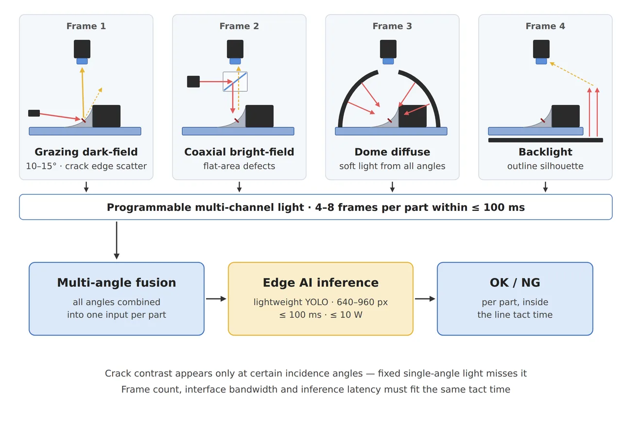
The figure shows four frames, grazing dark-field, coaxial bright-field, dome diffuse and backlight, lit and captured in sequence, then fused into one input on which edge AI decides OK or NG for each part. The programmable lighting box carries the target of 4 to 8 frames per part within 100 ms, and the inference box carries the targets of a 640 to 960 px input, 100 ms and 10 W or less. The backlight goes in only for outlines and through-holes; for fillet cracks the first three modes do the work.

Six frames in 100 ms choke the interface first

Turn the targets in the figure into bandwidth. Sending four 12.3 MB frames within 100 ms takes 491 MB per second, six frames take 737 MB and eight take 983 MB. At the 125 MB/s theoretical ceiling of 1 GigE a single frame alone takes 98 ms, and sending six frames within 100 ms uses 59 % even of 10GigE (1,250 MB/s). The real ceiling of multi-angle lighting is set by this bandwidth, not by the number of lighting channels.

Separating acquisition from transfer changes the numbers. Read the six frames off the sensor within 100 ms into the camera’s internal buffer, spread the transfer over the 0.5 second tact time⁵ of one part, and 147 MB per second, 47 % of 2.5GigE, is enough. The sensor then has to read 60 frames per second, though, and the camera buffer has to hold one part’s worth, 73.7 MB. I check those two conditions in the camera spec sheet first and choose the interface after. If the buffer falls short, the first frame of the next part pushes out the last frame of the previous one, so buffer capacity is counted in bytes, not frames.

Interface standards are moving the same way. On May 13, 2026, A3 officially released GigE Vision 3.0, stating that RDMA⁶ over RoCEv2 lets a camera write images straight into PC memory and that it adds an RDMA streaming protocol for 25GigE and above. Because the operating system no longer copies the images several times, the same PC keeps that much more headroom for inference.

A 960 px input erases a 30 μm crack

Lightweight detection models often take inputs shrunk to 640 to 960 px. Downsampling⁷ a 4,096 px image to 960 px is a 4.27-fold reduction, so one pixel becomes 42.7 μm and a 30 μm crack covers 0.70 pixels, less than a single pixel. At 640 px it is 0.47 pixels. The contrast recovered by six lighting frames gets averaged away in front of the model, and comparing only model accuracy while skipping this calculation leads to fixing the wrong thing.

Keeping the pixel count requires tiled inference⁸, cutting the image at native resolution. Cut into 960 px tiles without overlap, one frame becomes 5 tiles across and 4 down, 20 in all. Feeding each angle separately makes 120 tiles per part, and holding inference to 100 ms per part as the figure targets leaves only 0.83 ms per tile. Image fusion⁹, which merges the six frames into one input, brings that to 20 tiles at 5 ms each, so I make fusion the default and keep the per-angle images for root-cause analysis. Catching a crack that straddles a tile boundary requires the tiles to overlap by about a crack length, which adds tiles, so the overlap goes into the budget calculation too.

Choices on the model side keep growing. On January 14, 2026, Ultralytics released YOLO26, highlighting end-to-end inference without NMS and the removal of DFL, and stating that its nano model runs CPU inference up to 43% faster than YOLO11. That figure comes from the maker and the test hardware was not disclosed, so in my case I would set the 5 ms per tile budget by measuring the actual edge device at the same input size.

Setup and judgment conditions for solder crack detection

Three configurations go side by side on the same crack. The optics column keeps the camera and lens the same and changes only the lighting and the way images enter the model.

Configuration	① Minimum defect size	② Optics · lighting · WD	③ Algorithm parameters
Six multi-angle frames, fused input	Hairline crack 30 μm wide = 3 px (10 μm/px), lifted pad 80 μm = 8 px	4,096 × 3,000 px (3.45 μm pixels assumed), 25 mm lens at 0.345 magnification, about 98 mm from the lens center, WD confirmed against the spec reference plane, grazing 10 to 15° from four directions + coaxial + dome, six frames within 100 ms	Fuse the six frames into one input, 20 native-resolution tiles of 960 px, 5 ms per tile for 100 ms per part, minimum crack candidate length 6 px (assumed)
Six multi-angle frames, per-angle input	Same	Same camera and lighting, 73.7 MB buffer, sent over 2.5GigE during the 0.5 s tact (47 %)	120 tiles, 0.83 ms per tile. Combining per-angle results with OR piles a false-reject rate p per angle up to about 6p
One fixed ring-light frame (today)	Same	One ring-light frame, 12.3 MB sent over 1 GigE in 98 ms	Shrunk to 960 px, the crack covers 0.70 px. A crack that shows only at certain angles has no contrast even in the original

Laid next to each other, the rows show that the gain from more lighting angles survives only when interface bandwidth and inference budget come along with it. Shoot six frames and then shrink the input or judge each angle separately, and the contrast is either erased in front of the model or returns as false rejects. Conversely, for an inspection that only looks for voids on flat pads, one coaxial frame is enough and a six-frame setup just eats tact time and bandwidth. Which angle reveals a crack on solder fillets that mix curvature and gloss varies from lot to lot, so it cannot be guaranteed before a sample test.

An estimate that starts from four numbers

Multi-angle lighting and edge inference devices tend to be quoted separately, but the two share one tact time. Writing the crack pixel count, frames per part, transfer time and inference time per tile in one table lets you compare buying one more lighting channel, raising the interface by one class or changing the model input in the same units. With that table, the buyer can also read off which item is the bottleneck. This article explains technology and is not investment advice. See our Disclaimer.

Field Note

When catching solder fillet cracks with multi-angle lighting, I lay the six original frames, each lit at one angle, side by side and write down the ΔGV between crack pixels and the surrounding fillet for each angle. Seeing whether a crack buried at one angle appears at another decides how many angles go into the fusion, and every angle that can be dropped returns one frame’s share of the 100 ms budget. After that, I check on the same images how many pixels the crack keeps once the image is shrunk to the model input size.

Field Checkpoints

With the per-angle ΔGV and the crack pixel count at each input size written down, fill in the answers below before placing the order.

• Does the stacked height of the grazing ring, dome and coaxial unit fit within the lens WD? (About 98 mm from the center of a 25 mm lens; confirm again against the spec reference plane.)
• Can the sensor reach the frame rate to capture 4 to 8 frames within 100 ms? (40 to 80 frames per second at 12 MP)
• Has it been decided whether to finish transfer within 100 ms or buffer in the camera and send during the tact time? (73.7 MB for six frames)
• Has the number of pixels the smallest crack keeps at the model input size been calculated? (0.70 pixels when shrunk to 960 px)
• Is the per-part inference budget divided by the tile count longer than the latency measured on the actual device?
• Do the power and heat of the edge inference device fit the cooling conditions of the enclosure?
• Is there a schedule to re-measure the per-angle ΔGV whenever a new lot comes in?

Frequently Asked Questions

Wouldn’t raising the model input to 1,920 px solve it?

Shrinking 4,096 px to 1,920 px makes one pixel 21.3 μm, so a 30 μm crack covers 1.41 pixels. That still falls short of three pixels, and inference time grows with the larger input. Native-resolution tiles, or cropping only the areas around fillets, keep the crack’s pixel count.

Can’t each angle be judged separately and the results combined?

It can, but the number of judgments grows by the number of angles, and if a part is marked NG whenever any single angle flags a defect, the false rejects of every angle pile up. Fusing the six frames into one input lets the model see the relations between angles together and cuts the number of judgments.

Glossary

• [1] Multi-angle lighting programmable multi-angle lighting
  A method that controls light sources at several angles channel by channel and captures each frame under a different light. ↩
• [2] Edge AI edge AI
  Running inference on a device next to the line instead of sending images to a server. It cuts communication delay and data export. ↩
• [3] Grazing dark-field grazing dark-field
  Lighting that skims the surface at a low angle, keeping flat areas dark and lifting only spots that scatter light, such as crack edges. ↩
• [4] Coaxial bright-field coaxial bright-field
  Lighting from the same direction as the lens axis that images flat areas bright. Tilted or missing areas look dark. ↩
• [5] Tact time tact time
  The time the line allows for handling one part. Acquisition, transfer and judgment all have to fit inside it. ↩
• [6] RDMA remote direct memory access
  Writing data that arrives over the network straight into memory without copies by the operating system. ↩
• [7] Downsampling downsampling
  Reducing the pixel count of an image to make it smaller. Small defects get averaged with their surroundings and lose contrast. ↩
• [8] Tiled inference tiled inference
  Cutting a large image into pieces at native resolution and running inference on each piece. ↩
• [9] Image fusion image fusion
  Merging images taken under several lighting conditions into one input, by stacking them as channels or compressing their information. ↩

References

• A3, A3 Officially Releases GigE Vision 3.0, Opening New Possibilities in Machine Vision, 2026-05-13 (RDMA over RoCEv2, an RDMA streaming protocol for 25GigE and above) Read the release
• Ultralytics, Ultralytics YOLO26: The New Standard for Edge-First Vision AI, 2026-01-14 (end-to-end inference without NMS, DFL removed; the up-to-43% faster CPU inference of the nano model is the maker’s figure) Read the post
• Formulas: pixel resolution = defect width ÷ 3; view = pixel count × resolution; frame size = width × height × 1 B; bandwidth = frames × frame size ÷ time; reduction = original width ÷ input width; tile count = ⌈4,096 ÷ 960⌉ × ⌈3,000 ÷ 960⌉; ring height = radius × tan(angle of incidence); thin lens u = f × (1 + 1/m)
• Assumed values: a sensor with 3.45 μm pixels, a 25 mm lens, a 60 mm radius grazing ring, a 0.5 s tact, 100 ms of inference per part and a minimum crack candidate length of 6 px are assumptions for the worked example

Related reading — Where Do Fine Defects Go When You Shrink to 640 × 640? · In PCB Inspection, the Lens Comes Before the AI · Six Machine-Vision Lighting Methods and How to Choose