Machine Vision Lens Calculator — Catching the FOV Error the Shortcut Formula Hides, Plus Depth of Field and Diffraction in One Pass

OPTICS / CALCULATOR

The first formula most people reach for when choosing a lens is f = sensor size × WD ÷ FOV. One multiplication and one division give the focal length, and the focal length calculation article on this site starts from the same formula. The problem is that it is an approximation that holds only when the magnification is small enough. In a setup that images a 100 mm field with a 4096 px sensor, this approximation reports a FOV about 14% larger than reality.

The error is dangerous because it only shows up after the order is placed. If the approximation says “13% FOV margin” and a 25 mm lens is chosen, the real FOV at the same distance is about 1% narrower than the target and the edges of the part slide out of the frame. If the plan to widen depth of field by stopping down is then blocked by diffraction blur on small pixels, the lens, camera and mounting distance all have to be chosen again from the start.

The fix is to use the thin-lens formula together with two checks — minimum defect coverage in px and the Airy disk. The calculator below takes sensor pixel count, pixel size, FOV, object distance and aperture conditions, and computes the required focal length, pixel resolution, minimum defect coverage, depth of field and Airy disk diameter at once, then compares seven standard focal lengths at the same distance.

The approximation f = sensor × WD ÷ FOV computes a focal length exactly (1 + m) times too long, where m is the magnification.

1. Approximation vs. Thin-Lens Formula — The Gap Grows by the Magnification m

Point. The approximation gets worse as the magnification m grows. There is no need to memorize the size of the error: the overestimate ratio is the magnification m itself.

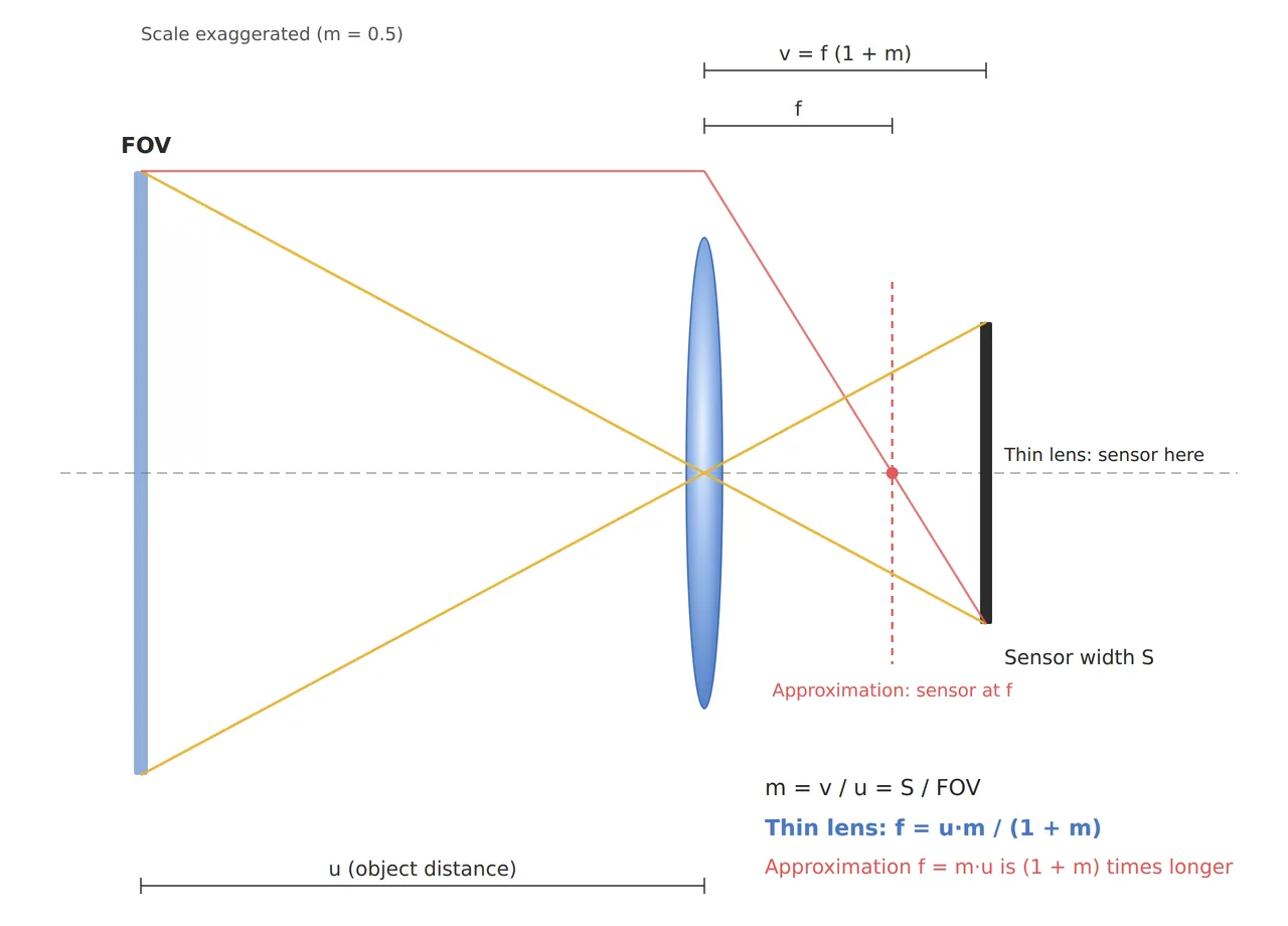
Reason. For a thin lens, object distance u, image distance v and focal length f satisfy 1/f = 1/u + 1/v, and the magnification is m = v/u = sensor width ÷ FOV. Solving the two gives f = u × m ÷ (1 + m), which means the image distance is v = f(1 + m). The approximation f = m × u assumes the sensor sits at the focal plane (v = f), so approximation ÷ exact = 1 + m. At a magnification of 0.064 the gap is 6.4%, at 0.141 it is 14.1%, and in high-magnification inspection near 1:1 (m = 1) it doubles.

Example. Re-solving the example from the focal length article (6.4 mm wide sensor, WD 200 mm, FOV 100 mm) with the thin-lens formula gives a magnification of 0.064 and a required focal length of 12.03 mm. The approximation gives 12.8 mm and leaves you torn between 12 mm and 16 mm, while the thin-lens formula shows that 12 mm is effectively the answer. At the same distance, however, the 12 mm lens gives a FOV of 100.3 mm, barely above the target, whereas the approximation computes 106.7 mm and makes it look as if there is margin.

Point. In setups where the magnification exceeds 0.1 — for example a 4096 px class sensor imaging 100 mm or less — do not finalize the lens with the approximation. Back-calculate the FOV with the thin-lens formula and confirm the final value with the lens maker’s FOV and WD data.

2. Resolution and Minimum Defect Coverage — Where It Breaks Before Focal Length

Point. Even with the right focal length, the setup fails if the minimum defect covers fewer than 3 px.

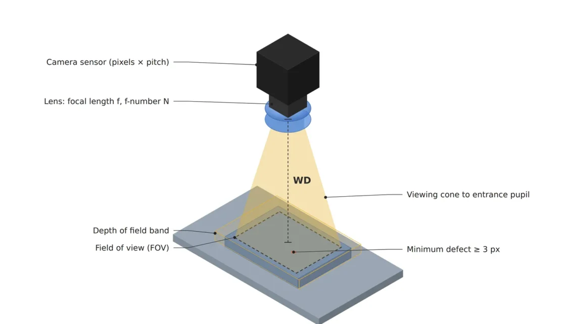
Reason. Object-side pixel resolution is set by FOV ÷ horizontal pixel count, and the common premise of the matching tables on this site is that the minimum defect must cover at least 3 px to be detected reliably (see the physics-first article). The focal length is only a means of producing the FOV; if the pixel count is short, no lens can create the resolution.

Example. A 1600 px sensor imaging a 100 mm FOV gives 62.5 µm/px, and a 100 µm defect covers only 1.6 px, which fails. Securing 3 px requires 33.3 µm/px or finer, i.e. at least 3,000 px across. Switching to a 4096 px sensor (3.45 µm pixels, 14.13 mm sensor width) gives 24.4 µm/px and about 4.1 px for the defect. The magnification then grows to 0.141 and the approximation’s overestimate grows to 14.1% as well. Raising the resolution makes the approximation more wrong. In fact, with a 25 mm lens at an object distance of 200 mm the approximation gives a FOV of 113.0 mm, but the thin-lens formula gives 98.9 mm, short of the target; the distance must be extended to about 202 mm to reach 100 mm.

Point. The calculation order is minimum defect → resolution → pixel count → focal length. Choosing the focal length first leads into the wrong loop of trying to fix a resolution shortfall by swapping lenses.

3. Depth of Field and Diffraction — What Stopping Down Gains and Loses

Point. Depth of field grows in proportion to the f-number, but on small pixels diffraction blur draws the limit first.

Reason. In the close-up approximation, total depth of field is DOF ≈ 2 × N × c × (1 + m) ÷ m² (N: f-number, c: circle of confusion, pupil magnification assumed to be 1). At the same f-number, the working f-number grows to Nw = N(1 + m), and the Airy disk diameter due to diffraction is about 2.44 × λ × Nw. The DOF formula covers geometric blur only, so once the Airy disk exceeds c the blur budget is already spent even at best focus and the real sharp range becomes narrower than the calculated value.

Example. With a 4096 px, 3.45 µm sensor, a 25 mm lens, an object distance of 202 mm (magnification 0.141) and a wavelength of 520 nm, taking c as 1 px (3.45 µm) at F8 gives a DOF of about 3.15 mm. But the Airy disk is then about 11.6 µm (3.4 px), more than three times c, so this 3.15 mm is a number that does not hold. Taking c as 2 px (6.9 µm) at F4 gives the same DOF of about 3.15 mm while the Airy disk of about 5.79 µm (1.7 px) stays inside c. The same DOF can be valid or invalid. Note that widening c to 2 px requires a corresponding margin in minimum defect coverage (about 4.1 px in this example).

Point. When raising the f-number to gain DOF, compare the Airy disk and c in the same table. If the part height variation exceeds the DOF, look at fixture height control or optical alternatives such as a telecentric lens or a variable-focus lens before raising the f-number.

4. Calculator — Focal Length, Resolution and DOF from Four Values

Fill in the eight input fields and the results table and the standard focal length comparison table are recalculated immediately. The defaults are the example conditions from the focal length article (1600 px, 4.0 µm pixels, FOV 100 mm, object distance 200 mm). Entering the second example (4096 px, 3.45 µm, FOV 100 mm, 202 mm, F4, c 2 px) leaves only the 25 mm row marked “OK” in the comparison table. The two pass criteria are FOV ≥ target and minimum defect ≥ 3 px.

The calculator uses the thin-lens approximation, and the inputs are computed only inside your browser and are not sent anywhere. The object distance u is measured from the lens principal plane, so confirm the real WD from the lens front to the object and the minimum object distance with the maker’s data.

5. Core Framework — Matching Table

Category	Item	Spec / Parameter	Basis / Note
① Minimum defect size	Minimum defect	100 µm	Design assumption. Covering at least 3 px is the detection premise
② Optical setup	Sensor	4096 px, 3.45 µm pixels, sensor width 14.13 mm	Calculated. 4096 × 3.45 µm
② Optical setup	Lens	Focal length 25 mm, F4	Thin-lens requirement 25.01 mm (u 202 mm)
② Optical setup	WD (working distance)	Based on object distance u of about 202 mm; confirm the real WD with maker data	u and WD differ with the principal plane position. Include lighting installation space
② Optical setup	FOV / resolution	FOV 100.0 mm, 24.4 µm/px	The approximation gives 114.2 mm, about 14% too large
② Optical setup	Depth of field	About 3.15 mm (c = 2 px = 6.9 µm)	DOF ≈ 2 × N × c × (1 + m) ÷ m²
② Optical setup	Diffraction	Airy disk about 5.79 µm (1.7 px) < c 6.9 µm	λ 520 nm assumed, Nw = 4.57
③ Algorithm	Defect coverage check	Minimum defect about 4.1 px ≥ 3 px	100 µm ÷ 24.4 µm/px
③ Algorithm	Size filter	Accept only components with a long side of 4 px or more	Back-calculated from ① (integer floor of 4.1 px)

Table insight. The moment the 4096 px sensor creates resolution margin (about 4.1 px), the magnification grows to 0.141 and the approximation’s FOV overestimate widens to 14%, so in this setup a choice that leans on the approximation produces “a shortfall that looks like margin”. And at the same DOF of about 3.15 mm, the F8 / c 1 px combination fails because of diffraction while only the F4 / c 2 px combination holds. Resolution, magnification, depth of field and diffraction are linked in one line — that is the point of this table.

6. Conditions Where the Opposite Approach Wins

• Dimensional measurement or parts with large height variation: choosing a telecentric lens, whose magnification stays nearly constant, comes before thin-lens calculations for an ordinary lens whose magnification changes with distance.
• Wide fields at several meters (magnification 0.01 or less): the approximation’s overestimate is 1% or less, so the approximation is enough.
• Zoom lenses or extension tubes, whose principal plane moves with each setting: calibrating the magnification by imaging a grid chart is faster and more accurate than calculation.

Final sharpness and defect contrast depend on the reflective properties of the target surface, so even when the calculation is right it cannot be guaranteed before a sample test.

Frequently Asked Questions

Q. When is the approximation f = sensor × WD ÷ FOV good enough?

Because the approximation’s overestimate equals the magnification m, decide first how much error you can accept. For example, if you need to stay within 1%, the approximation is enough only at a magnification of 0.01 or less, i.e. wide fields where the FOV is at least 100 times the sensor width.

Q. How many px should the circle of confusion c be?

There is no single answer; it is set by the margin in minimum defect coverage. If the defect barely exceeds 3 px, keep the blur budget tight at around 1 px; with a margin of 4 px or more, up to 2 px can be considered. Either way, check that the Airy disk is smaller than c.

Field Note

In a setup where a 25 mm lens had been chosen with the approximation, the left and right edges of the first frame came out narrower than the target FOV. At first I suspected lens tolerance or the sensor position, but recalculating with the thin-lens formula showed that at a magnification of 0.14 the approximation had inflated the FOV by nearly 14%. In the end we lengthened the mounting distance by a few millimeters, and that change forced the lighting bracket position to be redone as well. Since then I keep separate columns for the thin-lens FOV and the Airy disk in the review sheet before any order is placed.

Field Checkpoints

• Is the WD actually secured? — confirm with the maker’s FOV and WD table that the WD from the lens front, not the thin-lens u, is secured without interference from lighting or fixtures.
• Is the FOV calculated with the approximation even though the magnification m exceeds 0.1?
• Does the minimum defect cover at least 3 px (minimum defect ÷ pixel resolution)?
• Does the part height variation fit inside the calculated DOF, and is the Airy disk smaller than the circle of confusion c?
• Does the lens image circle cover the sensor, and is the calculated distance longer than the lens minimum object distance?
• For glossy surfaces, contrast cannot be guaranteed before a sample test even when the calculation is right — has it been confirmed with limit samples?

References

• Derivation of the Macro DOF equation — DOF = 2·c·N·(m + 1)/m² (pupil magnification assumed to be 1)
• Edmund Optics — System Throughput, f/#, and Numerical Aperture — (f/#)w ≈ (1 + m) × f/#
• Edmund Optics — The Airy Disk and Diffraction Limit — Airy disk ≈ 2.44 × λ × f/#

Related reading — How to Calculate Machine-Vision Lens Focal Length · The Tug-of-War Between Distortion Correction and Depth of Field: How Telecentric Lenses Catch Micro-Defects Without Losing Them · Machine-Vision Inspection: Physics Comes Before Software