Why Edge AI Vision Fails on the Factory Floor — A Troubleshooting Map from Symptom to Cause
EDGE AI / ALGORITHM
When an inspection model validated on a server is moved to an edge device, it usually runs well in the first week. The trouble starts a few weeks later, or in the afternoon, or on the day one more camera is added. Because it shows up as slightly lower accuracy or an occasionally late verdict, people look for the cause only inside the model.
If retraining starts before symptoms are linked to causes, the same symptom comes back even after weeks spent changing the model. When the cause lies outside the model — input resolution, heat, latency, bandwidth, lighting changes — retraining fixes nothing, and meanwhile the smallest defects escape quietly first.
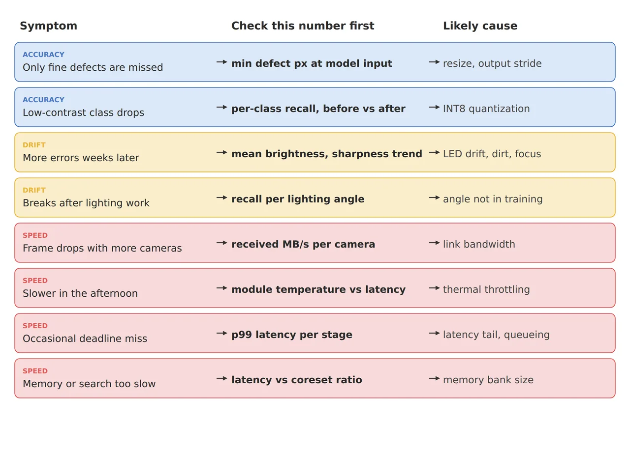
This article gathers the edge AI field failure causes covered separately on this site into one troubleshooting map in the order symptom → number to check first → likely cause → detailed article. The in-depth explanation of each cause is in the linked articles; here the aim is to decide where to look first for each symptom.
Retraining only works when the cause is inside the model. Check the physical quantity the symptom points to first.
1. Accuracy Symptoms — “Lower Than on the Server”, “Only Fine Defects Are Missed”
Point. If overall accuracy dropped by only 1 to 2 percentage points but one defect class disappeared, suspect quantization and input resolution first.
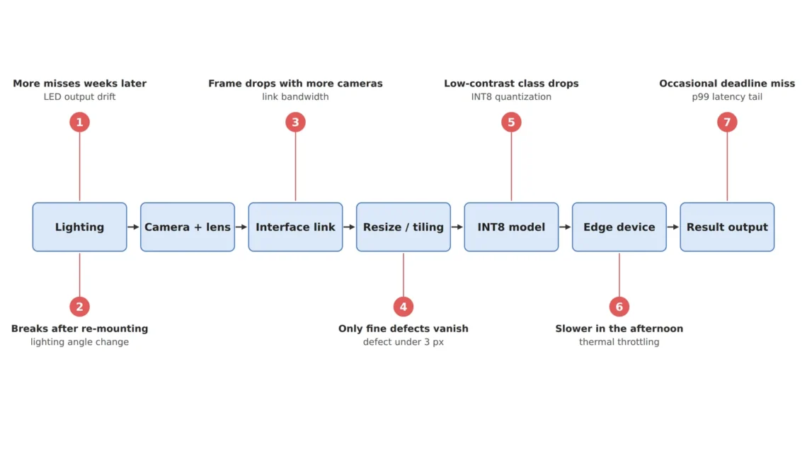
Reason. INT8 quantization divides a tensor’s value range into 256 steps, so defect signals with a small brightness difference from the background can merge into the same code (server vs. edge accuracy article, INT8 quantization article). Shrinking a high-resolution image to the model input size makes a defect that covered 3 px in the original fall below 1 px (tiled inference article). In both cases the average metrics barely show it.
Example. In the tiled inference article’s calculation, a 90 µm defect that covers 3 px at the original 30 µm/px disappears to 0.35 px in the 640 px downsampling path (256 µm/px). The knowledge distillation article shows how, at an output stride of 4 in a lightweight model, a 30 µm break falls to 0.75 cells.
Point. The numbers to check are per-class recall and minimum defect px at the model input. Do not start retraining before looking at these two values.
2. Speed Symptoms — “Slower Than the Benchmark”, “Occasionally Misses the Deadline”
Point. If it slows down in the afternoon, look at heat; if the average is fast but it is occasionally late, the latency tail; if frames drop after adding cameras, the interface.
Reason. A fanless device lowers its clock as the temperature approaches its limit, so inference time wavers (thermal design article); verdict latency is not one inference segment but the sum from trigger to output, so it must be viewed as p99 rather than the average (p99 latency budget article); and when several cameras share one link, bandwidth hits its limit first (interface bandwidth article).
Example. The p99 latency budget article points out that even when a 9 ms average inference time shows up, a delay on about 1 in 1,000 parts that exceeds the verdict deadline lets that part pass regardless of its verdict. The interface bandwidth article takes the effective limit of a 1GigE link as about 115 MB/s and follows how that limit shows up first in a configuration with several 12 MP cameras.
Point. The numbers to check are the time series of module temperature and inference time, p99 latency per segment and the actual received bandwidth per camera.
3. Symptoms That Appear Over Time — “More Errors Weeks Later”, “It Broke After Someone Touched the Lighting”
Point. If performance drifts slowly although the model has not changed, the input has changed.
Reason. Lens contamination, lighting degradation and focus drift leave traces in input statistics such as mean brightness and sharpness before they show in accuracy (input drift monitoring article), and LED light output loss progresses first in the direction of missed detections with no alarm (LED degradation article). A model that breaks after a lighting bracket is re-tightened has failed to learn a change of lighting angle, which brightness augmentation cannot imitate (limits of lighting augmentation article).
Example. In the LED degradation article’s example, an inspection that catches bright defects with an absolute gray-level threshold lets defects pass once the light output drops by 15%, because the defect signal falls below the threshold. The limits of lighting augmentation article proposes a capture matrix that holds out one azimuth to measure the recall drop under “lighting never seen before” as a number.
Point. The numbers to check are the trend of input statistics (brightness, sharpness) and recall per lighting condition. Start retraining when these two values point to the model as the cause.
4. Core Framework — Matching Table (Troubleshooting Map by Symptom)
| Category | Symptom | Number to check first | Likely cause · detailed article |
|---|---|---|---|
| ① Minimum defect size | Only fine defects are missed | Minimum defect px at the model input (3 px or more?) | Input resize — tiled inference / lightweight model stride — knowledge distillation |
| ① Minimum defect size | Recall drops only in low-contrast classes | Per-class recall before and after quantization | INT8 quantization — server vs. edge / INT8 quantization |
| ② Optical setup | More over-detections and misses weeks later | Mean brightness and sharpness trend | Lighting degradation, contamination, focus drift — input drift / LED degradation |
| ② Optical setup | Performance collapses after lighting work | Recall per lighting condition (azimuth, elevation) | Lighting angle change — limits of lighting augmentation |
| ② Optical setup | Frame drops after adding cameras | Received bandwidth per camera (MB/s) | Interface bandwidth — CoaXPress comparison / GigE Vision RDMA |
| ③ Algorithm | Slower in the afternoon, verdict jitter | Module temperature and inference time series | Thermal throttling — thermal design |
| ③ Algorithm | Fast on average but occasionally past the deadline | p99 latency per segment | Latency tail, queueing — p99 latency budget |
| ③ Algorithm | Out of memory, slow search | Latency and over-detection per coreset ratio | Memory bank size — memory-bank anomaly detection |
Table insight. Of the eight rows, retraining is the direct remedy only for lighting-angle generalization and lightweight model design; the rest start from settings and physical quantities outside training, such as the input resolution path, quantization settings, heat, latency, bandwidth and input degradation. Checking one number first for each symptom avoids much of the retraining loop — that is the point of this map.
5. Conditions Where the Opposite Approach Wins
- High-mix lines where products and defect types change often: a system that runs small-sample retraining quickly may come before cause analysis (few-shot anomaly detection article).
- Offline sample inspection with ample processing time: latency and heat items drop in priority.
- Environments where server inference is possible: quantization and thermal constraints disappear altogether, so first review “when cloud or server inference is the better choice” in the INT8 quantization article.
The weight of each cause changes with lighting and surface conditions, so which cause comes first cannot be guaranteed before a sample test.
Field Note
I once received a report that verdicts were occasionally late and started with model slimming, only to see two weeks later a log showing the module temperature hit its limit only in the afternoon. Had I first asked when the symptom appeared, it was a cause I could have confirmed on the first day. Since then, when a question comes in from the field, I ask for three logs — temperature, latency and brightness — before the model file. The table in this article follows that same order.
Field Checkpoints
- Does the WD keep its design value? — check first, because if the WD changes after reinstallation or a lighting replacement, the resolution and the defect px at the model input change with it.
- Does the minimum defect cover at least 3 px at the model input?
- Was per-class recall compared before and after quantization?
- Are p99 latency per segment and module temperature recorded on the same time axis?
- Is the received bandwidth of each camera within the effective link limit?
- Are input statistics (brightness, sharpness) computed on every frame — for diffusely reflecting surfaces, cannot be guaranteed before a sample test.
Related reading — It Worked Fine on the Server — Why Does Accuracy Drop on the Edge? · Where Do Fine Defects Go When You Shrink to 640 × 640? — Overlap, Boundary and Latency Design for Edge AI Tiled Inference · Is It Safe When the Average Latency Fits the Deadline? — Breaking Down the Edge Vision Inspection Latency Budget by p99 · Fast in the Benchmark, Why Slow by Afternoon? — Thermal Design and Sustained Inference for Fanless Edge Devices

Noctvision
A machine vision engineer who fits cameras, lenses, lighting, and image-processing algorithms together for a living. Years spent on continuous production lines, vibration, heat, and dust included, working through diffuse reflection, contrast, and resolution differences too fine for a spec sheet to capture inform every post here, closing the gap between theory and the shop floor. Off duty, that same eye for light and lenses goes into repairing fully mechanical vintage film cameras.


You May Also Like
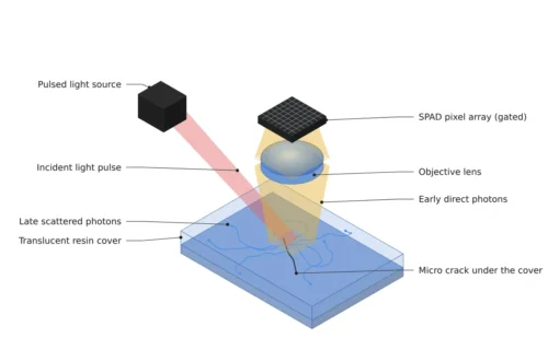
Does Extending the Exposure Solve It When Light Is Short? — How SPAD Sensors and Time Gating Rewrite Low-Light Inspection Design
What Should a Camera See When a Humanoid Grasps an Object?