On Reflective Surfaces, a Bilateral Filter Keeps the Crack a Gaussian Blurs Away

ALGORITHM

Put a 5×5 Gaussian over a 15 μm crack and its 20 GV contrast drops to 8.3 GV, while a bilateral filter with σ_range 10 keeps 16.1 GV.

Imaging particles and cracks on glossy molded housings and metal parts at 10 μm/px, I calculated how much defect contrast median, Gaussian and bilateral filters keep, and set the filter order from that.

About 11 min read

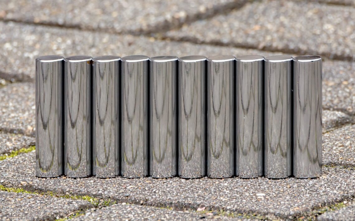
The targets are glossy molded housings and machined metal parts. Both surfaces have a strong specular component, so wherever the light falls, specular highlights¹ spread wide with brightness shooting up to 255, the top of the 8-bit range. The defects to find are 40 μm particles on the housing surface and 35 μm wide hairline cracks on the metal parts, with finer 15 μm cracks mixed in.

On such surfaces one filtering step can flip the result. Apply an ordinary smoothing filter over the highlights and the defect boundaries smear along with the noise, turning into missed detections; raise the sensitivity while leaving the noise and the highlight boundaries get picked up as defects, flooding the line with false rejects. Either way the cost comes back as defects leaking downstream or a stopped line.

When choosing a filter, I compare the contrast of one defect in GV before and after the filter. Run median², Gaussian and bilateral filters over the same defect in turn and write down the contrast each leaves, and which filter to apply in which order is settled more clearly than by feel.

No filter brings back a saturated pixel

The first step in the order is exposure, not a filter. Areas where highlights saturate³ are filled with the same value of 255, so the defect information inside them never existed, and no filter can create information that is not there. So I first set exposure and lighting angle so that the highlights of a good part stay below 255, cut out the remaining highlights with a mask, and only then apply filters. The principle that software cannot fill a gap in the optical setup takes its most concrete shape here.

Set the reference numbers. Viewing a 24.5 mm field with a camera 2,448 px wide gives 10 μm per pixel, so a 40 μm particle spans 4 pixels, a 35 μm crack 3.5 pixels and a 15 μm crack 1.5 pixels. The fine crack falls short of my rule of putting the smallest defect on three pixels or more, and catching it reliably would require shrinking the field to 12.2 mm or less. For these calculations I assumed a defect contrast of 40 GV for particles and 20 GV for cracks, and a noise standard deviation of 4 GV.

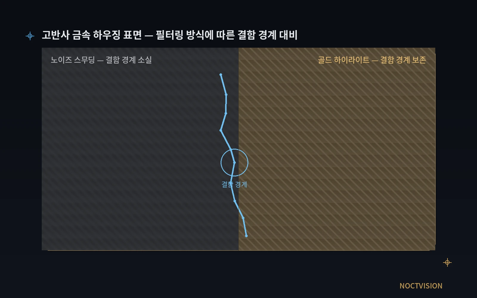
The figure draws the same housing surface under two kinds of processing. The left side is where noise was rubbed out evenly and the defect boundary blurred, and the right side is where the defect boundary survives as a line even within the highlights. The calculations below show that getting the right side depends on the size of the filter and the order in which it is applied as much as on its type.

Highlight boundaries pass straight through a bilateral filter

A bilateral filter⁴ lowers the weight of a neighbor not only by distance but also by brightness difference. A neighbor with a brightness difference Δ gets a weight of exp(−Δ² ÷ 2σ_range²), so across the 135 GV boundary between a 255 highlight and a background of 120, the weight is effectively zero at σ_range 10. The edge-keeping property leaves the highlight boundary razor sharp as well. Apply a bilateral filter before masking the highlights and that boundary passes straight on as a defect candidate.

The same formula also gives the rule for choosing σ_range. At the edge of a crack with 20 GV contrast, a neighbor’s weight is 0.135 at σ_range 10, 0.607 at 20 and 0.882 at 40. As σ_range grows past the defect contrast, pixels from across the edge mix in and the bilateral filter drifts toward a plain Gaussian filter⁵. I pick σ_range between the noise standard deviation and half the defect contrast, which for these conditions is 4 to 10 GV.

One kernel step of a median filter erases a particle

A median filter lines up the values inside its window and picks the middle one, so a defect that fills less than half the window disappears entirely. Calculating a 4-pixel particle with 40 GV contrast at shifting positions against the pixel grid, a 3×3 median leaves 36.8 to 40 GV, a 5×5 leaves 12.8 to 23.2 GV and a 7×7 leaves zero. One step of kernel size takes away half the contrast.

Long defects such as cracks hold out a little better. A crack 3.5 pixels wide keeps 32 to 40 GV after a 5×5 median, but at 7×7 it swings widely with position, between 12 and 32 GV. A crack 1.5 pixels wide already drops to 12 to 32 GV at 3×3 and to 0 to 12 GV at 5×5. In my case, I keep the median kernel smaller than the smallest defect, which under these conditions means 3×3.

Where a bilateral filter wins and where it loses

Add 4 GV of noise to a crack 1.5 pixels wide and run each filter 30 times, and the differences are clear. With no filter, the contrast is 19.9 GV and the contrast-to-noise ratio⁶ is 5.0; a 5×5 Gaussian (σ 1.5) cuts the noise to 0.88 GV but also trims the contrast to 8.3 GV, ending at 9.4. A bilateral filter with σ_range 10 keeps 16.1 GV of contrast for the highest ratio, 11.8, and raising σ_range to 40 brings it to 11.1 GV and 9.7, close to the Gaussian.

For a crack 3.5 pixels wide the ranking changes. The 5×5 Gaussian has the highest contrast-to-noise ratio at 18.3, and the bilateral filter with σ_range 10 reaches 13.9. In exchange, the edge width⁷ over which brightness climbs from 10 % to 90 % is 2.78 pixels for the Gaussian and 1.93 pixels for the bilateral filter, so if the crack width or position has to be measured, I choose the bilateral filter. For wide defects that only need a present or absent call, a Gaussian or a 5×5 median is enough, and the bilateral filter, which computes a weight for each of the 25 neighbors in its window, is 2.8 times heavier than a 3×3 median by neighbor count.

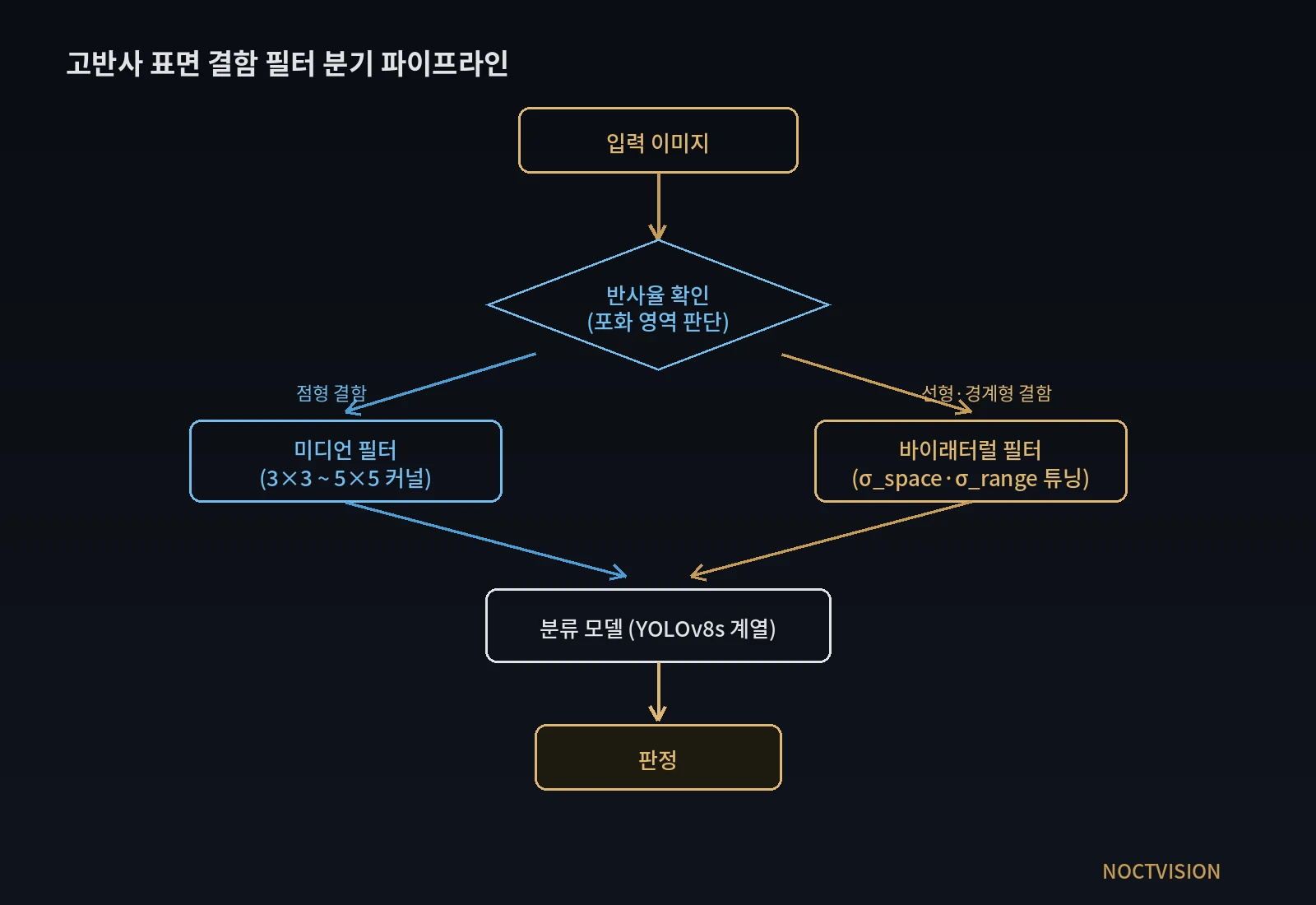
The flowchart in the figure checks reflectivity, then sends point defects to a median filter and linear or boundary defects to a bilateral filter before handing them to a classification model. Reflecting the calculations, two things need adjusting. Add a highlight masking step ahead of the branch, and of the 3×3 to 5×5 range in the median box, use only 3×3 for a 4-pixel particle.

A setup with the filter order settled, and its judgment conditions

The three defects go on the same camera with their filters and order laid out. Every row shares the same front end of exposure adjustment and highlight masking.

Defect	① Minimum defect size	② Optics · lighting · WD	③ Algorithm parameters
Particle on a molded housing (point)	40 μm across = 4 px (10 μm/px), 40 GV contrast assumed	2,448 px camera, 24.5 mm field, coaxial bright-field with low-angle dark-field as auxiliary, exposure set so normal highlights stay below 255, WD confirmed against the reference plane in the lens spec	Highlight mask → 3×3 median (a 5×5 leaves only 12.8 to 23.2 GV) → threshold
Hairline crack on a metal part (linear)	35 μm wide = 3.5 px, 20 GV contrast assumed	Same camera, coaxial bright-field	For a present or absent call, 5×5 Gaussian with σ 1.5 (contrast-to-noise ratio 18.3); to measure width, bilateral with σ_space 1.5 and σ_range 10 (edge width 1.93 px)
Fine crack (linear)	15 μm wide = 1.5 px, short of the three-pixel rule	Shrink the field to 12.2 mm or less, or raise magnification, to secure three pixels	Bilateral with σ_range 10 (keeps 16.1 GV of contrast); a Gaussian drops to 8.3 GV and a 5×5 median to 3.8 GV

Reading down the table, it becomes clear that the result is decided more by kernel size, σ_range and the order in which highlights are removed than by the name of the filter. Within the same median filter, the step from 3×3 to 5×5 costs half the particle’s contrast, and within the same bilateral filter, raising σ_range to 40 makes it hardly different from a Gaussian. Conversely, on a line where defects are mostly wide point-like stains and nothing needs measuring, a light pipeline built on a single median filter is better in both computation and delay. Whether these numbers hold on surfaces such as glossy housings, where the highlight position moves with every part orientation, cannot be guaranteed before a sample test.

Numbers to count again when moving on board

On-board processing⁸, which moves filtering and inference into the camera, cuts the transfer volume but shrinks the computation budget by the same token. A 5×5 bilateral filter over one 5 MP frame means about 125 million neighbor-weight calculations, so in my case I would set up a branch from the start that applies the bilateral filter only to zones with linear defects and handles the rest with a 3×3 median. If a new sensor shrinks one pixel from 10 μm to 7 μm, the same 40 μm particle spans 5.7 pixels, so the kernel size and σ_space have to be converted again in pixels. Leaving such numbers in the spec also lets the party placing the order see where the computing resources go. This article explains technology and is not investment advice. See our Disclaimer.

Field Note

When filters have to go on highly reflective parts, I lower the exposure to the point where normal highlights stay below 255, pick one defect in that image and write down its contrast in GV before and after filtering. Running 3×3 and 5×5 medians and bilateral filters with σ_range 10 and 40 over the same defect in turn puts how many GV each condition leaves on one line of a table. The judgment parameters are then set to avoid the condition that left the least.

Field Checkpoints

With the contrast left by each filter written in a table, hold the setup against the list below before it goes on the line.

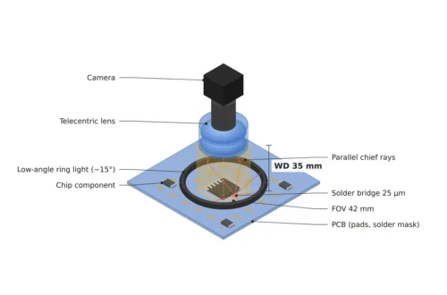
• Do the coaxial bright-field and the low-angle dark-field auxiliary light stay clear of each other within the lens WD? (Measure the WD from the reference plane in the lens spec.)
• Were exposure and lighting set first so that the highlights of a good part do not reach 255?
• Were the remaining highlight areas cut out with a mask before filtering?
• Is the median kernel smaller than the smallest point defect? (3×3 for a 40 μm particle at 10 μm/px)
• Is σ_range larger than the noise standard deviation and no more than half the defect contrast? (4 to 10 GV for 4 GV of noise and 20 GV of contrast)
• When the sensor or field changes, were the kernel size and σ_space converted again in pixels?
• Were public benchmark figures re-verified on in-house lot data? (Conditions of the conveying and alignment mechanism for the parts need a separate review.)

Frequently Asked Questions

Should the Gaussian filter be avoided?

It has its place. For defects wider than the window, such as a crack 3.5 pixels wide, judged only as present or absent, the 5×5 Gaussian gives the highest contrast-to-noise ratio, 18.3. The edge width spreads to 2.78 pixels, though, so for judgments that measure width or position, or for fine defects of 1.5 pixels, the bilateral filter is the one to use.

Can the accuracy figures in published papers be trusted as they are?

They are benchmarks obtained under specific lighting and imaging conditions, so they serve only as reference values. On highly reflective surfaces the highlight position changes with lot and orientation, so the numbers become shop-floor numbers only after being measured again on in-house lot data.

Glossary

• [1] Specular highlight specular highlight
  A very bright spot where a glossy surface mirrors the light source. With the wrong exposure, its pixels saturate at the top value. ↩
• [2] Median filter median filter
  A filter that lines up the pixel values in its window and replaces the center with the middle value. It is strong against point noise but erases defects smaller than half the window. ↩
• [3] Saturation saturation
  The state in which a pixel reaches the maximum brightness it can hold. In 8 bits, every brightness difference above 255 is recorded as the same value. ↩
• [4] Bilateral filter bilateral filter
  A filter that sets the weight of each neighbor from both distance (σ_space) and brightness difference (σ_range). It does not blend across edges with large brightness differences, which keeps them sharp. ↩
• [5] Gaussian filter Gaussian filter
  A filter that blends neighbors evenly with weights set by distance alone. It reduces noise well but spreads edges too. ↩
• [6] Contrast-to-noise ratio contrast-to-noise ratio, CNR
  Defect contrast divided by the standard deviation of the background noise. The larger it is, the easier a threshold separates the defect. ↩
• [7] Edge width edge width
  The distance over which brightness climbs from 10 % to 90 % across an edge. The narrower it is, the more precisely the edge position can be measured. ↩
• [8] On-board processing on-board processing
  Running filtering and inference on a processor inside the camera instead of on a separate PC. ↩

References

• Bilateral filter: C. Tomasi, R. Manduchi, Bilateral Filtering for Gray and Color Images, Proceedings of the IEEE International Conference on Computer Vision (ICCV), 1998, pp. 839–846
• Calculation method: a disk 4 pixels across and lines 1.5 and 3.5 pixels wide were drawn with 10-fold sub-pixels and averaged to 10 μm/px; 4 GV of noise was added 30 times each, then a SciPy median filter and OpenCV Gaussian (5×5, σ 1.5) and bilateral filters (d 5, σ_space 1.5, σ_range 10 and 40) were applied to calculate contrast, noise and edge width (10 to 90 %)
• Formulas: bilateral brightness weight = exp(−Δ² ÷ 2σ_range²); pixel resolution = field ÷ pixel count; contrast-to-noise ratio = contrast ÷ background noise standard deviation
• Assumed values: a 2,448 px camera with a 24.5 mm field, 40 GV particle contrast, 20 GV crack contrast, 4 GV noise standard deviation, and a 255 highlight on a background of 120 are assumptions for the worked example

Related reading — How Strongly Cross-Polarization Suppresses Glare Depends on the Lighting Angle · What HDR Multi-Exposure Fusion Does When Specular and Matte Share One Frame · How to Handle Imaging on Highly Reflective Surfaces