Overdetection or Missed Detection, Which One Costs More?

ALGORITHM

If one missed defect costs 100 re-inspections, the cheapest threshold pays 95 re-inspections a day to stop 1.6 escapes.

Taking a day of 10,000 plated terminals, I calculated where the costs of the two mistakes, the defect rate and a drifting light move the threshold.

About 11 min read

A nickel-plated connector terminal is close to a mirror, so its brightness changes sharply when the angle of the light shifts even a little. That is why it is shot under a dome light¹, which wraps the part in even light from all sides, to find pinholes 30 μm or larger where the plating is missing and the base shows through. The decision comes down to whether the defect score² crosses a preset threshold³, and that single threshold can keep the quality and production teams in meetings for weeks.

Lower the threshold and overdetection⁴, rejecting sound terminals as bad, grows until re-inspection staff have to be added. Raise it and escapes⁵, pinholed terminals passing through, grow until the customer finds the defects. The first cost goes out a little every day, the second goes out rarely but in large amounts. Unless the two different costs go on the same scale, the meeting tilts toward whoever talks loudest.

I end this meeting with three numbers: the cost ratio between one escape and one overdetection, the defect rate, and the way good and bad parts spread out in score. Assume 10,000 parts inspected a day, a defect rate of 0.3 %, and with one re-inspection costing 1, one escape costing 100.

Two mistakes hang on one threshold

An inspection decision falls into one of four boxes: the two where good is called good and bad is called bad, overdetection, where good is called bad, and an escape, where bad is sent on as good. Think of a smoke alarm: one that goes off at toast smoke has a lot of overdetection, and one turned down until it is quiet misses a real fire. There is only one sensitivity dial, so turning one side down turns the other up. Neither ever reaches zero.

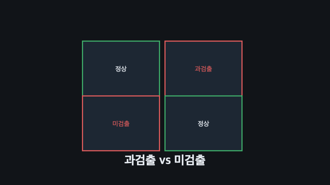
Decision \ Actual	Actually good	Actually bad
Called good	Correct	Escape (missed)
Called bad	Overdetection (re-inspection)	Correct

For an inspection that reduces the defect score to one number, this dial is the threshold. Assume good parts score in a normal distribution⁶ with mean 0.30 and standard deviation 0.08, and bad parts with mean 0.65 and standard deviation 0.10, and the two bell curves overlap around 0.45 to 0.55. Wherever the threshold goes, one of the overlapping tails crosses into the wrong box.

Put numbers on the costs and the threshold computes itself

Multiply the count of each mistake by its cost and add them, call the result the expected cost⁷, and the threshold belongs where that value is smallest. With costs at 1:1 the threshold settles at 0.583, giving 7.5 escapes and 2.0 overdetections a day for an expected cost of 9.6. Switch the costs to 100:1 and the threshold drops to 0.487; escapes fall to 1.6 a day but overdetections rise to 95, for an expected cost of 251.

Under the same 100:1 costs, keeping the 1:1 threshold of 0.583 raises the expected cost to 755, three times as much. Picking a threshold without agreeing on the cost ratio means paying that difference every day. In accuracy terms, 0.583 scores 99.90 % and 0.487 scores 99.03 %, so the threshold with the lower accuracy turns out to be the cheaper one. In my judgment, this gap is the first number to bring to a threshold meeting.

In the figure, the lowest point of the 100:1 curve sits on the stricter side of the 1:1 curve, the same direction in which the calculation moved 0.583 to 0.487. Where the bottom of the curve lies is not set by the cost ratio alone, and one more number pulls on that bottom.

The defect rate eats into the cost ratio

A 100:1 cost ratio makes it seem the threshold should drop hard, yet it only moves from 0.583 to 0.487. Of 10,000 parts a day, 9,970 are good and 30 are bad, so far more good parts than bad ones stand near the threshold. The cost ratio multiplied by the ratio of bad to good parts, 100 × 30 ÷ 9,970 = 0.30, is the weight that actually moves the threshold; the 100:1 cost ratio meets the 0.3 % defect rate and shrinks to 0.30.

If the defect rate rises to 3 %, the same cost ratio gives a weight of 3.09, the threshold drops to 0.435, and the line sees 449 overdetections and 4.7 escapes a day. The threshold is not a constant. On days when the defect rate climbs, the threshold has to be recalculated too. When the process settles and the defect rate falls, there is room to raise the threshold a little and cut re-inspections.

I put the cost ratio and the recent defect rate on one sheet for the threshold meeting. With only one of the two, the threshold cannot be calculated.

When the light dims 5 %, re-inspections grow 2.6 times

The calculation above stands on the premise that the score distribution is the same every day. Suppose the dome light’s LEDs age and dim by 5 %, and that pushes the mean good-part score from 0.30 to 0.33, up 0.03. The threshold of 0.487 stays put, yet overdetections rise from 95 to 244 a day, 2.6 times as many. The expected cost jumps from 251 to 400. The threshold did not change; the floor it rests on moved.

The wafer inspection equipment industry has its own word for this problem. Something the inspector reports as a defect but that is not really one is called a nuisance⁸. KLA Corporation’s Korean patent KR102203112B1 (Defect detection and classification based on attributes determined from a standard reference image; priority date February 6, 2014; granted January 13, 2021) uses a defect-free standard reference image to separate defects from nuisances. A golden image⁹ built from the median or average of several dies, histogram matching¹⁰ that fits each frame’s brightness distribution to the reference, and an image rendered from design data are listed as candidates for that reference.

The same patent uses attributes drawn from the test image, the difference image against the reference, and the reference image itself in its classification step. The reason for building the reference from many images shows in the arithmetic too. If pixel noise is Gaussian, a reference made from the median of 15 good parts carries about 32 % of the noise of a single image, and the noise of the difference image, the test image minus the reference, falls from 1.41 times single-image noise to 1.05 times. A quieter difference image narrows the good-part score distribution and shortens the overlapping tail. I would write the number of good parts behind the reference into the spec first.

Ending the threshold meeting with a calculation

Tying three things into one table at the setup stage shortens the meeting: how many pixels the defect occupies on screen, what holds that screen’s brightness in place, and what costs the threshold is chosen by. Assume a 2,448 × 2,048 px sensor with 3.45 μm pixels and a 25 mm lens, set the field of view at 24 mm across, and one pixel covers 9.8 μm on the terminal, with a WD¹¹ from lens to terminal of about 96 mm.

Item	① Minimum defect size	② Optical setup · WD	③ Algorithm parameters · in plain words
Pinhole decision	30 μm diameter = 3.06 pixels (9.8 μm/px)	Dome light, 25 mm lens, WD about 96 mm, field of view 24 × 20.1 mm	Threshold of 0.487 at the lowest expected cost (100:1 cost ratio, 0.3 % defect rate assumed). 1.6 escapes and 95 re-inspections a day
Brightness watch	Reference only, so no defect size	Gray reference patch in a corner of the field, same lens and WD	Correct before judging when patch brightness drops 5 %. A 0.03 shift in good-part scores raises re-inspections to 244 a day
Reference image	The baseline that fixes the decision coordinates	15 good parts shot with the same setup	A pixel-wise median reference cuts difference-image noise from 1.41 to 1.05 times. Match each lot’s histogram to the reference

Only when the three rows connect from top to bottom does a threshold chosen by cost keep the same meaning in the next lot.

There are also places where raising the threshold is right. If a missed terminal gets caught again by a full inspection in a later process before reaching the customer, or if the flaw is cosmetic and the customer does not object, the escape cost falls far below 100 and the threshold rises toward the 1:1 point. If a second camera handles re-inspection cheaply, the overdetection cost shrinks instead and the threshold can go lower. I note such conditions next to the cost ratio. How far the score distribution strays from the assumed shape as the plating gloss varies from lot to lot cannot be guaranteed before a sample test.

Calculating the threshold from costs is the fastest way for an inspection algorithm engineer to get on the same page as the quality team, and quality control and process engineering use the same formula. For the buyer, setting the labor cost of 95 re-inspections a day beside the claim cost of 1.6 escapes tells more than the accuracy figure on an inspection spec sheet. This article explains technology and is not investment advice. See our Disclaimer.

Field Note

To set the threshold for this terminal line, I would first pull the mean and standard deviation of good-part scores from a day of inspection records. I check how far they stray from the assumed 0.30 and 0.08, then reshoot the same 50 terminals with the dome light dimmed by 5 % to see whether the mean moves by about 0.03. If that shift is large, I add a step that corrects brightness with the reference patch in the corner of the field before touching the threshold.

Field Checkpoints

Once a day of records and the 50 reshot terminals have checked the distribution assumptions, the questions below turn the threshold into spec-sheet sentences.

• Is a WD of about 96 mm (25 mm lens, 24 mm field of view) available after adding the dome light height? (whether the dome fits between the lens and the terminal)
• Have quality and production agreed on a numeric cost ratio between one escape and one overdetection? (whether 100:1 or 10:1 changes the threshold)
• Have the recent defect rate and defect counts by type gone into the threshold calculation? (whether 0.3 % and 3 % split the threshold into 0.487 and 0.435)
• Are daily re-inspections and escapes counted separately at the chosen threshold? (instead of overall accuracy)
• Is lighting brightness logged on every frame with the reference patch in the corner of the field? (whether a 5 % drop multiplies re-inspections by 2.6)
• How many good parts went into the reference image? (a median of 15 gives difference-image noise of 1.05 times)
• Has the score distribution been rechecked with samples from lots with different plating gloss?

Frequently Asked Questions

Isn’t an accuracy above 99 % enough?

On a line with a 0.3 % defect rate, passing every terminal as good already scores 99.7 % accuracy. In the calculation above, the 1:1 threshold scores 99.90 % and the 100:1 threshold 99.03 %, yet under 100:1 costs the more accurate one costs three times as much. In inspections with a low defect rate, the cost only shows when daily escapes and re-inspections are counted separately in place of accuracy.

Once set, is the threshold done?

It gets recalculated whenever the cost ratio, the defect rate or the score distribution changes. If the defect rate rises from 0.3 % to 3 %, the threshold drops from 0.487 to 0.435, and if the lighting wobbles and the good-part distribution shifts, re-inspections grow even at the same threshold. That is why it pays to record the three numbers behind the threshold along with the threshold itself.

Glossary

• [1] Dome light dome illumination
  Lighting that bounces light inside a hemispherical cover to illuminate a part evenly from all sides. It spreads out the hotspots on shiny surfaces. ↩
• [2] Defect score anomaly score
  A single number the inspection algorithm gives each image or location for how defect-like it is. The text uses a range from 0 to 1. ↩
• [3] Threshold decision threshold
  The cutoff value above which a defect score is judged as a defect. ↩
• [4] Overdetection false positive, overkill
  The mistake of judging a good part as bad. It costs re-inspection labor and time. ↩
• [5] Escape false negative, missed detection
  The mistake of passing a bad part as good. Found by the customer, it comes back as claims and lost trust. ↩
• [6] Normal distribution Gaussian distribution
  A bell-shaped distribution symmetric around its mean. About 68 % of values fall within one standard deviation of the mean. ↩
• [7] Expected cost expected cost
  The sum of each mistake’s count multiplied by its cost. The threshold goes where this value is smallest. ↩
• [8] Nuisance nuisance defect
  A detection the inspector reports as a defect that is not really one. The wafer inspection term for overdetection. ↩
• [9] Golden image golden reference image
  A reference image built by combining several defect-free images pixel by pixel with a median or average. ↩
• [10] Histogram matching histogram matching
  A correction that reshapes one image’s brightness distribution to match that of a reference image. ↩
• [11] WD working distance
  The distance from the lens to the surface being inspected. The value in the text uses a thin-lens approximation measured from the lens center. ↩

References

• KLA Corporation, Korean patent KR102203112B1, Defect detection and classification based on attributes determined from a standard reference image (priority February 6, 2014; filed February 5, 2015; granted January 13, 2021. Nuisance discrimination, median or average references from multiple dies, histogram matching, references rendered from design data, combined attributes from test, difference and reference images)
• Formulas: expected cost = C_escape × escapes + C_overdetection × overdetections, escapes = bad parts × Φ((t − μ_bad) ÷ σ_bad), overdetections = good parts × (1 − Φ((t − μ_good) ÷ σ_good)), weight that moves the threshold = cost ratio × bad parts ÷ good parts, median reference noise ≈ σ × √(π ÷ 2n), difference-image noise = √(σ² + reference noise²)

Related reading — Deep Learning vs. Rule-Based Algorithms, When to Use Which · When the Light Dims by 5 %, How Many Good Pixels Turn Into Defects? · Adding Reasons to an AOI Defect Call with a Vision Language Model