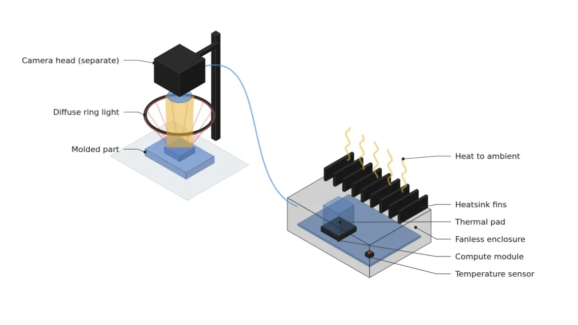
Fast in the Benchmark, Why Slow by Afternoon? — Thermal Design and Sustained Inference for Fanless Edge Devices

EDGE AI / THERMAL DESIGN

An inspection system with an edge inference module inside a fanless enclosure usually shows excellent numbers in pre-shipment testing. Power it on and run a benchmark for a few minutes, and the inference time is constant and the decision latency does not waver. The problem is that after it is installed on the line and a few hours pass into the afternoon, the decision latency starts to become erratic. Nothing has changed in the model or the optical setup, yet the results differ.

The cause of this phenomenon is mostly thermal throttling. As the module temperature approaches its limit, the compute clock drops, and as the temperature falls, it rises again. As the clock rises and falls, the inference time rises and falls with it, and this fluctuation (jitter) creates a tail in which the decision signal misses the deadline. Parts that miss the deadline pass regardless of the decision, so the thermal problem ultimately returns as defect escapes and re-inspection cost. Without logs, even the fact that the cause is temperature never comes to light.

The solution is to define inference performance in thermal equilibrium rather than in a cold-start benchmark. First calculate the steady-state temperature from thermal resistance and the thermal time constant, fix the power mode and clock to guarantee a floor of performance instead of a ceiling, and record temperature, clock and latency together so that the cause of jitter can be traced.

The real inference speed of an edge device is measured not right after power-on but after it reaches thermal equilibrium.

1. Why a Cold-Start Benchmark Cannot Show the Steady State

Point. Thermally speaking, a benchmark lasting a few minutes looks at only the very beginning of the rise curve.

Reason. The module, heatsink and enclosure have a mass that stores heat (heat capacity C) and a path that releases heat to the ambient air (thermal resistance R). When a constant power P is applied, the temperature rise follows the form 1 − e^−t/τ, and the thermal time constant τ is R × C. The final rise is set by P × R, but reaching that value takes several multiples of τ. A fanless structure has a large R and, with its aluminum mass, a large C as well, so τ easily falls in the range of tens of minutes.

Example. As design assumptions, take a module power of 15 W, an enclosure thermal resistance of 2.5 °C/W, a heat capacity of 600 J/°C and an ambient of 40 °C. τ is 2.5 × 600 = 1,500 s, or 25 min, and the steady-state temperature is 40 + 15 × 2.5 = 77.5 °C (calculated). Yet the rise at the 5 min benchmark point is only 1 − e^−0.2 ≈ 18% of the final value, staying at about 46.8 °C. The benchmark sees performance in the cool state, while the line sees performance in the hot state.

Point. Performance verification must start after continuous operation of at least 3τ (95% of the final rise). Inference time measured without this condition is not a basis for design.

2. How Thermal Throttling Creates Decision Jitter

Point. The damage from throttling comes less from slowing down itself than from repeatedly speeding up and slowing down.

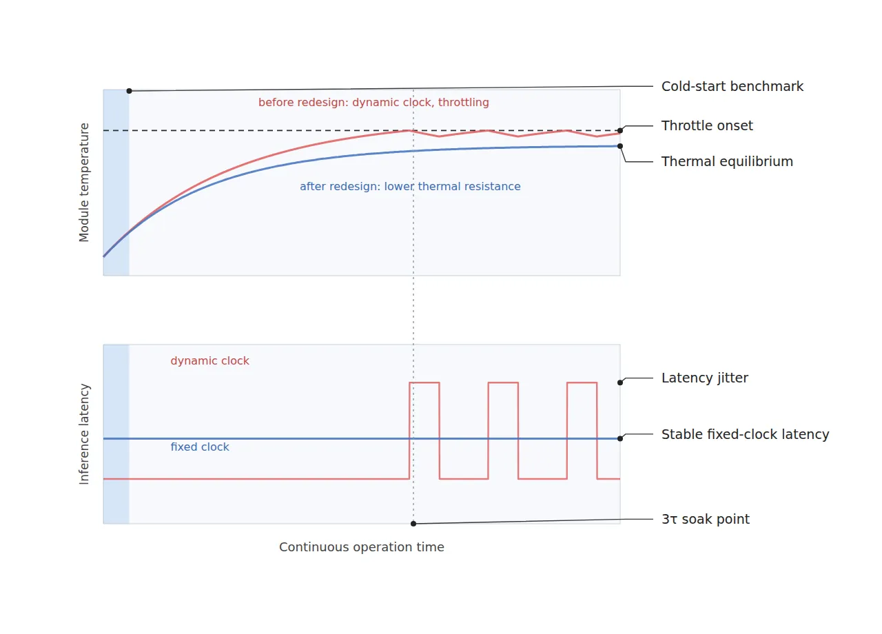
Reason. Thermal protection logic lowers the clock near the limit and raises it again when the temperature falls. Inside an enclosure with a long thermal time constant, this control creates a slow oscillation, and the inference time, inversely proportional to the clock, oscillates along with it. The decision latency distribution splits into two peaks, and p99 lands on the slow peak. Looking only at the average, it seems merely a little slower, but from the deadline point of view the slow state becomes the reference.

Example. For a model with an inference time of 10 ms, if throttling lowers the clock to 70%, the inference time becomes 10 ÷ 0.7 ≈ 14.3 ms (calculated). If the clock swings between the two states, the same model shows a fluctuation of 4.3 ms. Conversely, if the clock is fixed at 85% from the start, the inference time is 11.8 ms; the average is slower but the fluctuation disappears. In an inspection bound by a deadline, a fixed 11.8 ms is a better design than a wavering 10 to 14.3 ms.

Point. Therefore the power mode and clock must be fixed not at maximum performance but at a value sustainable in thermal equilibrium. Dynamic clock scaling is a convenience feature, not the default for inspection equipment.

In an inspection with a deadline, a fixed slowness is safer than a wavering speed.

3. Heat Dissipation Design and Temperature Logging — Making Heat a Calculable Variable

Point. The starting point of heat dissipation design is not the heatsink size but a one-line calculation: allowable thermal resistance R_max = (target temperature − maximum ambient) ÷ power.

Reason. The throttling onset temperature is set by the module manufacturer’s documentation, but the design target temperature should be set with a margin below it. Once the target temperature, maximum ambient and fixed power are decided, the thermal resistance the enclosure must satisfy follows directly. On top of that come thermal pad contact, fin orientation and the convection conditions at the installation location. If the camera head is placed in the same enclosure, thermal expansion of the lens barrel can shift the focus, so as a principle the camera is kept outside the thermal path of the compute module.

Example. With a target temperature of 70 °C, a maximum ambient of 40 °C and a power of 15 W, R_max is (70 − 40) ÷ 15 = 2.0 °C/W. The earlier 2.5 °C/W enclosure exceeds this condition, so the fin area must be increased or the installation location changed. Once 2.0 °C/W is achieved, τ becomes 2.0 × 600 = 1,200 s (20 min), and verification operation needs 3τ = 60 min or more. During operation, module temperature, clock, power and inference time are recorded at 1 s intervals on the same timestamp.

Point. The value of the temperature log lies in post-hoc analysis. When a latency tail appears, the clock value at the same moment must be immediately comparable, so that thermal problems can be separated from software problems. Software optimization cannot fully cover defects in the optical setup or the thermal design.

4. Core Framework — Matching Table

Category	Item	Specification / Parameter	Basis & Notes
① Minimum defect size	Black speck (foreign matter) on molded part surface	Diameter 90 µm or more	Design assumption. Occupies 3.0 px at 30 µm/px
① Minimum defect size	Flash at the parting line	Width 150 µm or more	Design assumption. Occupies 5.0 px
② Optical setup	Illumination	Diffuse ring light, 45° incidence from above	Based on matte resin. Glossy resin requires re-review of diffuse reflection conditions
② Optical setup	Sensor & lens	2048 × 1536 px (pixel pitch 3.45 µm), focal length 16 mm	Design assumption. Magnification 0.115× (calculated)
② Optical setup	WD (working distance)	140 mm or more must be secured	Thin-lens approximation object distance about 155 mm (calculated). Measure including ring light thickness
② Optical setup	FOV & pixel resolution	FOV 61.4 mm × 46.1 mm, 30 µm/px	2048 px × 30 µm = 61.44 mm (calculated)
② Optical setup	Camera placement	Installed separately from the compute enclosure	Avoids focus shift from lens barrel thermal expansion
③ Algorithm	Power mode & clock	Fixed at 15 W, clock fixed at 85% (dynamic scaling disabled)	Design assumption. Inference constant at 11.8 ms (calculated)
③ Algorithm	Thermal design criterion	R ≤ 2.0 °C/W, τ = 20 min	(70 − 40) ÷ 15 = 2.0, 2.0 × 600 J/°C = 1,200 s
③ Algorithm	Verification run	Measure after 60 min or more of continuous operation, jitter p99 − p50 ≤ 3 ms	3τ = 95% of the final rise
③ Algorithm	Temperature logging	1 s interval, temperature, clock, power and inference time recorded in sync, warning at 65 °C	Target 70 °C − 5 °C margin

Table implication. The 90 µm black speck in ① is 3.0 px at the 30 µm/px of ②, leaving no margin in optical resolution. In such a configuration, if heat reaches the camera side and the focus shifts even slightly, the contrast of a 3 px defect collapses first. Meanwhile, the 15 W power and R of 2.0 °C/W in ③ reach exactly the 70 °C target at steady state, so at an installation location where the ambient is higher than the design assumption, the margin becomes zero. Thermal design margin must be calculated and managed in the same way as optical resolution margin.

5. When the Opposite Approach Wins

• Installation environments where forced air cooling is allowed: If there are no dust or maintenance constraints, a fan structure lowers thermal resistance substantially, so the fixed clock value can be set higher. Managing the filter replacement cycle is a prerequisite.
• Intermittent inspection: If inspection runs for only a few minutes at a time with long idle periods in between, τ is never reached, so cold-start performance is close to actual operating performance.
• Offline inspection with a loose decision deadline: If latency fluctuation does not lead to defect escapes, raising average throughput with dynamic clock scaling can be the better choice.

For materials with strong diffuse reflection such as glossy molded parts, the preprocessing load and power conditions change with the illumination and exposure conditions, so the thermal design figures above cannot be confirmed before sample testing.

Field Note

I once traced a phenomenon in a fanless inspection unit installed near a high-temperature roll section, where the decision latency tail grew long only in the afternoon. I suspected the software first, but when I overlaid the 1 s interval temperature and clock log on the latency records, the clock had dropped by one step at every moment a tail appeared. After fixing the clock at a lower value and changing the fin orientation, then measuring again after 60 min or more of operation, the average became slightly slower but the jitter dropped noticeably. Results may differ where the ambient conditions of the installation location differ, so I do not state this as certain.

Field Checkpoints

• Is a WD of 140 mm or more secured by measurement — verify including the ring light thickness and the bracket for separate camera installation.
• Has the surface material and reflectance of the target been identified first — illumination and preprocessing conditions differ depending on whether the resin is matte or glossy.
• Was the performance measurement made in thermal equilibrium, after continuous operation of 3τ or more.
• Was the allowable thermal resistance R_max calculated from the maximum ambient at the installation location.
• Are the power mode and clock fixed, and are they restored to the same values after a reboot.
• Are temperature, clock, power and inference time recorded at 1 s intervals on the same timestamp.