In the Age of Deep-Learning Inspection, What to Check Before Camera Spec

EDGE AI

In a 30 μm crack inspection, the numbers to set before choosing a camera are 10 μm/px, a 1.25 mm depth of field, and a model input size that splits one frame into 35 tiles.

Taking an SMT board that mixes metallic gloss with matte resin, I followed one unbroken chain of calculation from defect size through magnification and depth of field to edge inference time.

About 10 min read

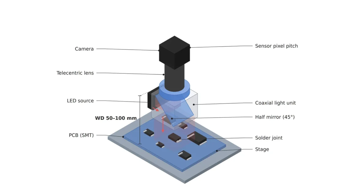
One SMT board mixes several surfaces with very different properties. The solder and component leads have a metallic gloss that throws light back in one direction, the resin bodies of the parts are matte and scatter light, and the green solder mask sits somewhere in between. Assume a setup that hands a deep learning¹ model the job of finding micro-cracks around 30 μm wide, foreign particles, and bridges joining neighboring leads on this surface.

Pick the model by name first and fit the camera later, and training data piles up with cracks imaged at under two pixels or with the warped half of the board out of focus. A model built from that data does well in the demo and falls apart under the line’s worst conditions, and the boards that slip through in the meantime come back as field claims.

I run the order the other way around. From the defect size I calculate the pixel resolution, then the magnification and depth of field, and last the model’s input size and the inference time on the edge device. The camera and the model are chosen from the candidates that satisfy those numbers.

The defect size sets the magnification

My rule is to cover a 30 μm crack with at least three pixels, so one pixel must not exceed 10 μm on the board. Assuming a 4,096 × 3,000 px sensor with 3.45 μm pixels, the lens magnification² is 3.45 ÷ 10 = 0.345, and one frame sees 41.0 × 30.0 mm. With a telecentric lens³, whose magnification is fixed, this number does not wobble with distance, so parts of different heights image at the same size. The WD⁴ from lens to board is a fixed value for each model of this lens, so it is confirmed on the spec sheet.

The camera’s pixel count comes out as a result of this calculation. At the same 0.345 magnification, a sensor 2,448 px wide narrows the field of view to 24.5 mm and adds shots per board, while more pixels cut the number of shots. Fix the pixel count first and the relationship flips, which easily produces a setup that gains a wide field of view while the crack drops below two pixels.

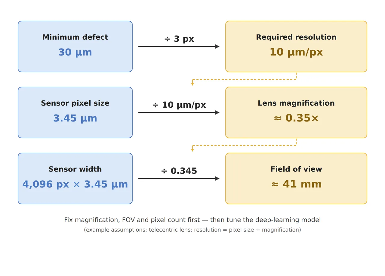
The flowchart in the figure links these three steps with arrows. It starts at the defect size and comes down through resolution, magnification and field of view in that order, with the camera spec left at the bottom as something to check. Keeping this order also settles which numbers on a camera spec sheet deserve a look first.

One aperture stop decides whether board warp stays covered

Once the magnification is set, the depth that stays in focus, the depth of field⁵, follows. Take the permissible circle of confusion⁶ as two pixels, 6.9 μm, and assume an f-number⁷ of f/8, and the depth of field at 0.345 is 2 × 8 × 6.9 μm × (1 + 0.345) ÷ 0.345² = 1.25 mm. Opening up one stop to f/5.6 shrinks it to 0.87 mm.

The board is not flat. Assume a board warp of 1 mm, and it fits inside the 1.25 mm at f/8 but overflows the 0.87 mm at f/5.6. On tiles in the overflow, crack edges spread across two or three pixels, and although they look similar to a person, they become different images to the model. Stopping down to f/8, on the other hand, lets in half the light of f/5.6, so at the same exposure time the lighting has to be twice as bright. The metallic glossy surfaces are better lit evenly from straight on with coaxial illumination⁸, but the resin bodies stay correspondingly dark. I would keep f/8 as the default and look at brighter lighting first.

Feed the whole frame into a 640 px input and the crack disappears

The model has a resolution too. Assume a detection model that takes a 640 × 640 px input, shrink the whole 4,096 px frame into it, and the width drops to one 6.4th, turning a 30 μm crack that spanned three pixels into 0.47 pixel. A trace smaller than a pixel blends into its surroundings during the shrink and disappears, so the 10 μm/px the optics fought for collapses to 64 μm/px at the model’s entrance.

That is why the frame is cut at full resolution into 640 px pieces, a method called tiling⁹. A 4,096 × 3,000 px frame splits into 7 tiles across and 5 down, 35 per frame, and since neighboring tiles have to overlap a little so cracks on tile borders are not missed, the real count runs higher. This is why the input size is the very first question when choosing a model.

700 tiles set the time on the edge device

Take the board as 160 × 100 mm and overlap frames by 10 %, and you get 5 frames across and 4 down, 20 frames in all. With 35 tiles per frame, 700 tiles pass through the model for each board. Assuming inference on one tile takes 8 ms on the edge device¹⁰, that is 5.6 seconds, and with a 10-second tact time, 4.4 seconds are left for capture and transfer.

The floor on the tile count is set by board area and pixel resolution. One 640 px tile is a 6.4 mm square on the board, so covering 160 × 100 mm directly in board coordinates takes 25 × 16 = 400 tiles. Of the 700, 300 are the share lost to frame overlaps and to leftover tiles at frame edges. Stitching the frames into board coordinates and then re-cutting the tiles brings inference down to 3.2 seconds, but the stitching has to be more precise than the crack width. I do not lock in the edge device spec until this calculation is done.

Training data is collected after the optical setup is done

Deep learning classification learns from images taken under slightly varying light and judges more forgivingly than one fixed threshold. That forgiveness only applies when the crack is in the image, though; a model cannot create a crack that is not on screen. It is like a lens that has lost focus: changing the film does not make the image any sharper. So collecting training images starts only after the three rows below are settled.

Item	① Minimum defect size	② Optical setup · WD	③ Algorithm parameters · in plain words
Micro-crack, bridge	30 μm wide = 3 pixels (10 μm/px)	Telecentric 0.345×, 4,096 × 3,000 px at 3.45 μm, field of view 41.0 × 30.0 mm, coaxial light. WD confirmed as the lens spec’s fixed value and checked against the install space with the light housing height added	Feed the frame as 35 tiles of 640 px without shrinking it. Cut tile borders with overlap
Board warp	1 mm warp assumed	Depth of field 1.25 mm at f/8 (6.9 μm circle of confusion assumed), 0.87 mm at f/5.6. f/8 needs twice the light	Log a sharpness score with every tile to flag tiles outside the depth of field
Inference time	Tile count is the variable	160 × 100 mm board, 20 frames (10 % overlap)	700 tiles × 8 ms = 5.6 seconds (assumed). Re-cut in board coordinates: 400 tiles, 3.2 seconds. Measure on the edge device

Only images taken after the three rows are settled teach the model the shape of the defect without teaching it the wobble of light and focus.

Some inspections do not need the optics tightened this far. If the defects are large, several hundred μm or more, such as a missing part or reversed polarity, a regular wide-field lens and a shrunk input are enough, with plenty of depth-of-field margin. Conversely, if the cracks are finer than 30 μm or the board warp exceeds 1 mm, the setup moves on to shooting several images at split focus positions on top of the telecentric lens and tiling. How much coaxial lighting will lift crack contrast on a surface that mixes metallic gloss and resin cannot be guaranteed before a sample test.

The chain that runs from defect size through magnification, depth of field and model input to inference time is a problem worth working by hand for anyone preparing to become a vision engineer, and for the side buying the equipment, whether that chain has any break says more about an inspector’s real ability than its camera pixel count or AI model name. This article explains technology and is not investment advice. See our Disclaimer.

Field Note

To bring up this setup, I would start by measuring board warp. I measure ten production boards with a displacement sensor to see whether the maximum warp stays within 1 mm, and if it exceeds that, the 1.25 mm depth of field at f/8 is not enough, so I look at a setup that shoots at split focus positions. At the same time I cut one 4,096 px frame into 35 tiles of 640 px, run them on the edge device, and measure whether inference per tile stays within the assumed 8 ms.

Field Checkpoints

Once the warp of ten boards and the inference time of 35 tiles have checked the assumptions, I move on to the questions below.

• Does the telecentric lens’s fixed WD, plus the coaxial light housing height, clear the install space? (checked against the WD value on the lens spec sheet)
• Is a 30 μm crack held in three pixels or more (10 μm/px or finer)?
• Does the maximum warp of production boards fit inside the depth of field of the chosen aperture (1.25 mm at f/8)?
• Has the model input size been checked, and is the frame split into tiles instead of shrunk? (shrunk to 640 px, the crack becomes 0.47 pixel)
• Does the tile count per board times inference time per tile fit within the tact time? (700 tiles × 8 ms = 5.6 seconds)
• Were the training images taken after the light, lens and aperture were settled?
• Has crack contrast been checked with samples where metallic gloss and resin mix?

Frequently Asked Questions

Doesn’t a camera with more pixels solve everything?

With the same pixel size, more pixels only widen the field of view one frame covers; at the same magnification, the pixel resolution stays the same. Raising the magnification to sharpen resolution shrinks both the field of view and the depth of field, so on a warped board more area falls out of focus. Either way, the number of tiles passing through the model per board is set by area and resolution, so the inference time has to be calculated along with it.

Wouldn’t a larger model input remove the need for tiling?

Enlarging the input to 4,096 × 3,000 px lets the frame go in without shrinking, but computation grows roughly with input area, to about 30 times that of a 640 × 640 px input. Whether it fits in the edge device’s memory, and how its time compares with processing 35 separate tiles, is decided by measuring both on the same device.

Glossary

• [1] Deep learning DL
  A multi-layer neural network approach that learns its own decision criteria from many example images. ↩
• [2] Magnification magnification
  The size of the image on the sensor divided by the real object size. At 0.345, 10 μm on the object becomes 3.45 μm on the sensor, one pixel. ↩
• [3] Telecentric lens telecentric lens
  A lens whose magnification barely changes when the object moves back and forth within a set range. Used for dimensional measurement and for parts at different heights. ↩
• [4] WD working distance
  The distance from the front of the lens to the surface being inspected. For a telecentric lens, this distance is fixed by design. ↩
• [5] Depth of field DOF
  The range of depth that stays sharp in front of and behind the focus distance. It widens as the aperture is stopped down. ↩
• [6] Circle of confusion permissible circle of confusion
  The diameter up to which a point blurred by defocus is still treated as sharp. The text sets it at two pixels. ↩
• [7] F-number f-number
  Focal length divided by the diameter of the lens opening. Stopping down one stop from f/5.6 to f/8 cuts the incoming light roughly in half. ↩
• [8] Coaxial illumination coaxial illumination
  Lighting sent down the same axis as the lens through a half mirror. It lights flat, shiny surfaces evenly. ↩
• [9] Tiling tiling
  Cutting a large image at full resolution into pieces the size of the model input, so small defects do not vanish in a shrink. ↩
• [10] Edge device edge device
  A compact computer that runs the model right beside the inspection line, with no server. Its memory and compute are limited, so inference time has to be measured. ↩

References

• Formulas: pixel resolution = minimum defect width ÷ 3, magnification m = pixel size ÷ pixel resolution, field of view = pixel count × pixel size ÷ m, depth of field ≈ 2 × N × c × (m + 1) ÷ m², light ratio = (N₁ ÷ N₂)², defect width after shrink = original pixels × input width ÷ frame width, tiles = ⌈frame width ÷ 640⌉ × ⌈frame height ÷ 640⌉, compute ratio ≈ ratio of input areas

Related reading — Where Do Fine Defects Go When You Shrink to 640 × 640? · Why the Faintest Scratch Disappears First Under INT8 Quantization · Four Snags in Initial Jetson Orin Nano Setup