When 3D+AI Inspection Answers the Shape Defects 2D Can’t Catch

ALGORITHM

A chip part lifted by 20 μm leaves almost no trace in a photo taken from above, yet a camera viewing a laser line at 30° reads it in 3.9 μm steps.

On a board that mixes black epoxy with glossy solder, I calculated where 2D ends and 3D begins, including the shadows and noise that appear once you switch to 3D.

About 10 min read

The body of a chip part on a PCB is black matte epoxy that sends back almost no light, while the solder at both ends is glossy metal that throws light back in one direction. Assume the job is to find a part with one end lifted by 20 μm, leaving the solder joint under-formed. In a 2D photo taken from above, this part looks almost exactly like a normal one.

A lifted part can pass the electrical test before shipping and fail later in the field, where repeated vibration and heat break the joint. Training a 2D deep learning model further does not create height information that is not in the photo, so this defect keeps passing as good. Because it surfaces at the customer, tracing the cause back takes time as well.

SICK announced that it has added a 3D inspection capability combining height-data analysis with deep learning to its Nova software (metrology.news, August 11, 2026). According to the report, training runs directly on the inspection device with no extra computing hardware. I work out when this pairing of 3D and AI pays off by calculating first on the optical side that produces the height data.

A photo from above knows nothing of height

What a 2D camera measures is the amount of light that reaches each pixel. Surfaces that send back the same amount of light appear equally bright in the photo even at different heights, and a surface with low reflectance¹ such as black epoxy barely changes in brightness when lifted by about 20 μm. Laying the light low to look at the shadow cast by the lifted end is another option. At a light elevation of 10°, the shadow of a 20 μm step is 113 μm long, several pixels, but on black epoxy the shadow is as black as the background, so it shows almost no contrast. Height leaves no mark on brightness.

On a map, it is the difference between a satellite photo and contour lines. A satellite photo shows mountains and plains only as colors, and height can only be read once contour lines are drawn separately. The height map² a 3D sensor produces plays the role of those contour lines, recording for each pixel how many μm the surface stands up, regardless of brightness.

View the laser at a slant and height turns into position

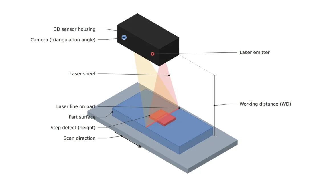
Among the ways to build a height map, one widely used on production lines is laser triangulation³. A laser line is drawn straight down onto the part, and a camera views that line from a slanted angle. When the surface rises by Δz, the line shifts sideways on the camera image by Δz × sin θ (θ being the angle between the laser plane and the camera’s line of sight), and that shift is converted back into height. That is the whole principle.

Put a camera whose pixel covers 15.6 μm on the part (2,560 px across a 40 mm field of view, assumed) at 30°, and the height that shifts the line by one pixel is 15.6 ÷ sin 30° = 31.3 μm. Assuming subpixel⁴ precision of one-eighth of a pixel, reading the center of the line from its brightness profile, the height resolution is 3.9 μm, a fifth of the 20 μm lift. With my rule of a third of the target step, 6.7 μm or finer, 30° passes. Narrow the angle to 15° and one pixel becomes 60.4 μm, or 7.5 μm at one-eighth of a pixel, which misses the rule.

Steeper angles stretch the shadow

A steeper angle sharpens resolution but adds places the camera cannot see. Because the camera looks at a slant, the area behind a tall part is hidden from its line of sight, and the hidden length is part height × tan θ. Behind a 2 mm tall electrolytic capacitor, 1.15 mm becomes shadow⁵ at 30° and 2.0 mm at 45°. A small 0.6 mm wide chip part sitting inside that zone drops out of the height map entirely.

Shadows can be reduced with a camera on each side of the laser filling in each other’s shadows, or by lowering the angle and making up the lost resolution with subpixel precision. The first doubles the camera cost, and the second needs samples to confirm the subpixel assumption actually holds. I would first measure the gaps between tall and small parts on the drawing and count how many spots have a gap narrower than the shadow length.

Glossy solder punches another hole. If the laser bounces off in one direction only, by specular reflection⁶, and misses the camera, that spot comes back empty; if it hits the camera head-on, the pixels saturate⁷ and the center of the line cannot be read. Black epoxy is the opposite: too little light calls for longer exposure, yet getting a profile every 50 μm along the travel direction at 100 mm/s takes 2,000 profiles a second, so each exposure has to finish within 0.5 ms. Setting the travel speed itself needs a separate review.

With 5.12 million points, noise rises like a defect

The first step in finding a lift on the height map is fitting the board’s reference plane. The board itself is warped and tilted, so a plane is fitted to areas without parts, and viewed as the residual⁸, the amount that departs from that plane, the 20 μm step rises above the tilt. The obstacle is noise in the residual. Assume height noise with a standard deviation of 2 μm and a threshold at half the lift, 10 μm, or five times the noise, and the chance that a single point crosses the threshold on noise alone is 2.9 in 10 million.

It looks small, but one height map holds 2,560 × 2,000 = 5.12 million points, so about 1.5 noise points per map rise like defects. That is why a single threshold is not the end of it: a minimum-area condition is layered on, keeping a candidate only when 5 or more points connect. I set that minimum area at about a quarter of the profiles a lift spans. A 20 μm lift spanning 1 mm shows up in 20 consecutive profiles at 50 μm spacing along the travel direction, so this condition does not erase it.

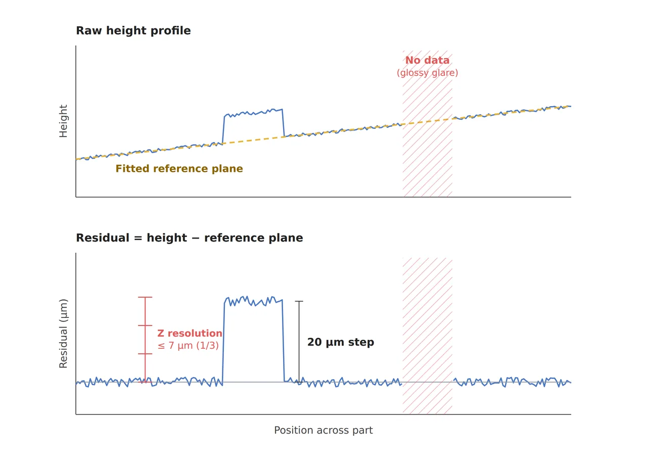
The figure is a concept drawing of a 20 μm step emerging in the residual after a reference plane is fitted to a tilted raw height profile, together with a band where glossy reflection left no data. If a defect falls inside that empty band, no residual appears however well the plane is fitted. Software can only work with the places that have values.

What the AI on top of the height map adds

The AI on top only has work to do when the height map holds the defect. The AI comes second. Defects that show up in height, such as a lift or a missing part, are largely filtered by the residual and the minimum area, and the AI spends its effort separating real defects from normal variation among those candidates. Feed in the 2D appearance photo together with the height map, and one model sees both defects without height, such as smeared printing, and defects without a brightness difference, such as a lift. The article only says training uses representative good and defective parts, so how many images are enough is something to confirm for each defect type.

The sensor’s WD⁹ and measuring range differ by model, so they are confirmed on the spec sheet, leaving clearance above the tallest part and the board warp. The table below lists, row by row, the share that optics and algorithms each take on to catch a single lift.

Item	① Minimum defect size	② Optical setup · WD	③ Algorithm parameters · in plain words
Lift (height)	20 μm high, 1 mm or longer (needs height resolution of 6.7 μm or finer)	Laser triangulation, camera at 30°, 15.6 μm pixel, 3.9 μm with one-eighth subpixel assumed. WD and measuring range confirmed on the sensor spec, clearance above 2 mm parts	Residual threshold of 10 μm after plane fitting (5× an assumed 2 μm noise), candidates only when 5+ points connect. Classify with the 2D photo and the height map together
Shadow (occlusion)	1.15 mm behind a 2 mm part (30°)	Add a camera on the opposite side, or lower the angle and make up with subpixel reading	Mark missing areas with a mask and log them as excluded from judgment. Check parts inside them separately
Profile spacing	50 μm along the travel direction	2,000 profiles a second at 100 mm/s, exposure 0.5 ms or less. For black epoxy, calculate laser power and exposure together	Confirm a 1 mm lift spans 20 profiles. Travel speed control needs a separate review

The thresholds and AI in the third column only mean something once the first row sets the height resolution, and the shadow in the second row is a place no algorithm can fill.

2D still comes out ahead in some cases. Defects without any change in height, such as color or print condition, are fine with 2D, and on lines where gathering 3D profiles takes longer than the tact time, 3D becomes a burden. If the target step falls short of three times the sensor’s height resolution, switching to 3D still leaves the defect buried in noise. How much data will go missing on a board that mixes glossy solder and black epoxy cannot be guaranteed before a sample test.

Calculating height resolution and shadow from a single angle is arithmetic a 3D vision engineer does every day. It needs only sin and tan, so it is a good one to work by hand when you are first learning the inspection-equipment side. For the side investing in the equipment, whether the ratio of target step to sensor height resolution exceeds 3, and how much shadow area is left excluded from judgment, say more about real detection power than the labels 3D and AI. This article explains technology and is not investment advice. See our Disclaimer.

Field Note

To add 3D inspection to this board, I would scan one board without lifts 20 times at the same spot and start by measuring the standard deviation of the residual. If it exceeds the assumed 2 μm, the arithmetic that makes the 10 μm threshold five times the noise falls apart, so I reset the angle and exposure. Next I pick out on the drawing the parts sitting within 1.15 mm behind the tall capacitors and log the missing-data ratio at those spots separately.

Field Checkpoints

Once 20 scans and a drawing check have tested the noise and shadow assumptions, only the questions below are left.

• Are the 3D sensor’s WD and measuring range secured with clearance above the tallest part (2 mm) and the board warp? (whether there is room for the sensor at that height)
• Is the height resolution 6.7 μm or finer against the 20 μm target step? (calculated from the angle and the subpixel assumption)
• Has the number of parts to inspect inside the shadow behind tall parts (1.15 mm at 30°) been counted?
• Has the residual noise standard deviation been measured from 20 scans of the same board? (compared with the 2 μm assumption)
• Has it been confirmed that the 5-connected-point condition does not erase a 1 mm long lift?
• Has the missing-data ratio at glossy solder spots been checked on sample boards?

Frequently Asked Questions

How do structured light and laser triangulation differ?

Structured light projects a pattern such as stripes over the whole area and calculates height over a wide region at once, which suits parts that are standing still. Laser triangulation builds the height map one profile at a time, which suits capturing parts while they move. Both work by viewing at a slant, so shadows and data loss on glossy surfaces come with either one.

With a height map, can the 2D photo be dropped?

Defects without height, such as color, printing or stains, do not appear in a height map. Some sensors provide a reflected-brightness image along with height, but it is brightness captured at a single laser wavelength, so it cannot separate color differences the way a 2D color camera can. If appearance defects are among the inspection items, keeping the 2D photo alongside is the safer choice.

Glossary

• [1] Reflectance reflectance
  The share of light hitting a surface that comes back out. Black epoxy has low reflectance, so it images dark even under the same light. ↩
• [2] Height map range image
  An image that stores a height value for each pixel in place of brightness. 3D sensors produce it. ↩
• [3] Laser triangulation laser triangulation
  A method that calculates height from how far a laser line shifts on the image of a camera viewing it at a slant. ↩
• [4] Subpixel subpixel
  A calculation that reads a position finer than one pixel from the shape of the brightness profile. How finely it reads depends on noise and line shape, so it needs to be confirmed. ↩
• [5] Shadow occlusion
  The area behind a tall object hidden from a slanted camera’s line of sight, where height values go missing. ↩
• [6] Specular reflection specular reflection
  Reflection from a smooth surface in which light bounces off in one direction only, at the same angle it arrived. ↩
• [7] Saturation saturation
  The state in which a pixel reaches the brightest value it can hold and cannot tell brighter light apart. ↩
• [8] Residual residual
  How far the actual height departs from the fitted reference plane. Used to remove board warp and tilt and leave only defects. ↩
• [9] WD working distance
  The distance from the front of the sensor or lens to the surface being measured. A 3D sensor only measures height within a set range around this distance. ↩

References

• metrology.news, SICK brings AI-powered 3D machine vision to industrial inspection with Nova (August 11, 2026. Deep learning combined with height-data analysis, training on the inspection device, no extra computing hardware, training with representative good and defective parts)
• Formulas: height resolution = pixel resolution ÷ sin θ × subpixel ratio, shadow length = part height × tan θ, cast shadow = step ÷ tan(light elevation), noise exceedance (5σ, one-sided) ≈ 2.87 × 10⁻⁷, noise points per map = points × exceedance, profile rate = travel speed ÷ profile spacing

Related reading — How 3D Structured Light Measures a Solder Lead Lift That Brightness Cannot Show · The Defect Zone You Miss When You Switch to 3D Inspection · Deep Learning vs. Rule-Based Algorithms, When to Use Which