Why the Faintest Scratch Disappears First Under INT8 Quantization

EDGE-AI

In INT8 quantization the faintest scratch vanishes first because the brightest reflection sets the step size.

Taking a plated connector-pin detector moving onto an edge camera, I calculated how much the average metric hides, how large one step is, and how many samples it takes to confirm the loss.

About 16 min read

PCB connector pins are plated with gold or tin, so they give off specular reflection¹ close to a mirror’s. Under coaxial illumination² the flat plated face sends light straight back into the lens and turns nearly saturated, while a scratch about 20 μm wide scatters the light sideways and stays behind as a thin dark line. Moving the detector that looks for this scratch from FP32 on a server to an INT8 quantization³ model on an edge smart camera usually goes smoothly. Inference gets faster and the overall metric hardly changes, so it is easy for the floor to conclude there is no problem.

The trouble shows up weeks later. Only the faintest scratches slip through as escapes in certain lots, and tracing them back shows the model’s overall performance intact while recall⁴ has dropped in a single defect class that had low contrast to begin with. Why would the faintest defect go first? I follow that question with three numbers: how much the average metric hides the loss, how large one INT8 step is, and how many scratch samples it takes to confirm the loss.

Averages move only 0.3 points

Take a validation set of 2,000 images and assume 40 of them (2 %) contain a faint scratch. If the FP32 model catches 38 of the 40 for a recall of 0.95 and the INT8 model catches only 32 for 0.80, missed scratches grow fourfold, from 2 to 8. With every other class judged the same and FP32 overall accuracy put at 99.0 %, INT8 lands at 98.7 %, a shift of just 0.3 points. The average dilutes six lost images across 2,000.

The average is this dull because of how the classes are made up. A validation set holds far fewer defect samples than normal ones, and faint scratches are a minority again within the defects. Overall accuracy and mAP follow the many normal images and the high-contrast defects, so a drop in a minority class sinks below the decimal point. That is why I put the single overall line and the per-class recall table on the same page when I compare a model before and after quantization. The go or no-go for production comes from the per-class table.

One step’s size comes from the brightest value

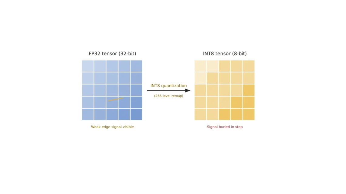
INT8 quantization moves activations, once held in FP32, into integers between -127 and 127. The number that sets how much real value one integer step stands for is the scale factor⁵, and in the simplest symmetric scheme it is the largest absolute value seen in the calibration⁶ images divided by 127. Think of a ruler whose spacing is cut to fit the longest object it will ever measure. A difference much smaller than one mark never shows on that ruler.

In an image of plated pins, that maximum rarely comes from the scratch. Early-layer activations spike hardest where brightness changes most, at a highlight on the flat plating or a glint⁷ on the edge of a pin. Assume that maximum is 24.0 and the faint scratch produces a response of 0.09 in the same channel, and one step comes to 24.0 ÷ 127 = 0.189. The 0.09 falls short of half a step, 0.0945, so it rounds to 0 and the trace of the scratch is wiped out in that layer.

Generalize the calculation and one criterion comes out. When the response a defect produces in a layer is smaller than 1/254 of that layer’s largest activation, symmetric INT8 rounds it to zero. On a screen where the glint spikes about 267 times higher than the scratch, the scratch already stands on that border. Later layers may make up part of the loss, yet the weaker a defect’s signal, the less material there is to make it up with.

Drawn as one picture, the path from camera to edge device through inference, and the class where recall falls off along the way, looks like this. Transfer and inference happen to every class alike, yet the loss gathers in the one class with low contrast, because that class carries the smallest responses into every rounding step.

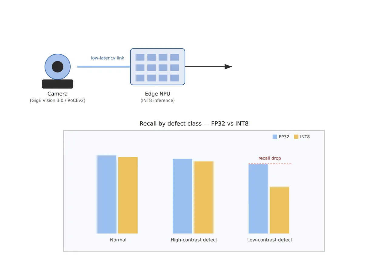
The figure shows recall falling in the low-contrast class alone as images pass through transfer and inference. By the calculation above, the size of that loss depends on the maximum that sets the step, and that maximum can be changed. There is one way to change it on the software side and one on the optical side.

Clip the glints and the scratch gets four steps

Setting the step at the boundary that cuts off the top 0.01 % of activations, in place of the maximum, is percentile calibration⁸. Assume the 99.99th percentile in the same layer is 3.0; one step becomes 3.0 ÷ 127 = 0.0236, and the scratch response of 0.09 survives as four steps (0.0945). The error is 5 %, and every glint above 3.0 is clipped to 3.0. Glint brightness plays no part in the defect decision, so I see this trade as a good deal in most cases.

How much of the range to clip, though, has a different answer for each network. A paper that NVIDIA and Georgia Tech researchers released in April 2020 (Wu et al., arXiv:2004.09602) compared max, entropy⁹ and several percentile calibrations across many networks. Max calibration gave inconsistent quality from network to network, which the authors put down to outlier values, and the 99.9 % percentile clipped large values so hard that accuracy dropped sharply on most networks. The best results came from entropy, 99.99 % and 99.999 %, yet the paper concludes that no single calibration is best for every network.

The same paper advises that if no calibration reaches the accuracy target, the next step is partial quantization¹⁰, which leaves some layers unquantized, or quantization-aware training. Carried over to the plated-pin model, the order becomes clear. I would build one INT8 model with each of the four, max, entropy, 99.99 % and 99.999 %, and rank them by the recall of the faint-scratch class instead of the overall metric. If all four fall short, I would test a build that keeps the early layers, where the scratch response first forms, in FP16.

Plating reflections widen the quantization range

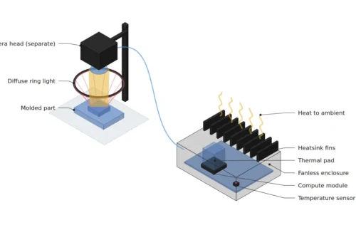
Clipping by percentile ends in software, but the glints that need clipping are made by the lighting and the plated surface in the first place. Under coaxial light a flat plated face looks bright and even, while on a bent pin or a rounded edge only the narrow band that faces the lens head-on sends light back, and that band saturates easily. Those bands push up the maximum in every calibration image and make the steps coarse.

Lowering the maximum with lighting changes the outcome even under the same max calibration. Assume a diffuser on the coaxial light or a dome light spreads the highlights, and exposure set below saturation halves the largest activation from 24.0 to 12.0: one step becomes 0.0945, and the scratch response of 0.09 survives as one step. Combined with percentile calibration, the margin grows further. If the scratch’s own contrast is buried under noise in the raw image, though, no calibration can create that signal. How far the glint maximum swings as plating thickness and surface roughness vary from lot to lot cannot be guaranteed before a sample test.

The idea of building differing value distributions into quantization design also appears in patent literature. Intellectual Discovery’s US patent US12335477B2 (Neural network feature map quantization method and device; priority date November 18, 2020; granted June 17, 2025) states in its abstract that the feature maps a multilayer neural network produces are quantized according to the network’s structure or the feature map’s attributes. The description gives examples such as whether the sample-value distribution is closer to uniform, Gaussian or Laplace, and classes grouped by channel or spatial similarity. Read against the plated-pin model, it says the channels where glints gather and the channels where the scratch response lives should each get a ruler of their own.

How many images per-class recall takes

Even with a per-class table, few samples make the numbers wobble. Catching 38 of 40 scratches gives a recall of 0.95 with a 95 % confidence interval¹¹ of 0.83 to 0.99 by the Wilson method, and catching 32 gives 0.80 with 0.65 to 0.90. The two intervals overlap between 0.83 and 0.90, so 40 images leave it unclear whether INT8 cut recall by 15 points or chance made the difference. Forty images are too few.

Raise the scratch samples to 140 and the picture changes. Catching 133 gives 0.95 with 0.90 to 0.98, and catching 112 gives 0.80 with 0.73 to 0.86, so the two intervals separate. Working out by normal approximation how many images it takes to read recall near 0.9 within ±5 points also gives 1.96² × 0.9 × 0.1 ÷ 0.05² ≈ 139. I set 140 images per faint defect class as the floor of the validation set. Until that many real defects have gathered, I would keep the INT8 model out of production decisions.

The calibration set follows the same principle. The range is measured on the calibration images, so a set of clean samples with few glints sets a range narrower than the real line, and production images may then clip large values the decision depends on, such as pin outlines. My rule is a calibration set of images exactly as the line shoots them, with the same lens, the same WD¹² and the same lighting settings.

What to fix so a 20 μm scratch survives

Tying three things into one table at the setup stage shortens the spec meeting: how many pixels the defect occupies, what holds down the brightest value on screen, and what criterion picks the quantization. Set 6.67 μm per pixel so a 20 μm wide scratch spans 3 px, assume a 2,448 × 2,048 px sensor with 3.45 μm pixels, and the field of view is 16.3 × 13.7 mm at a magnification of 0.52×. With a 25 mm lens plus about 13 mm of extension tube, the thin-lens approximation puts the pin about 73 mm from the principal plane of the lens; the actual WD is measured from the front of the lens and comes out shorter, so it has to be checked against the lens datasheet.

Item	① Minimum defect size	② Optical setup · lighting · WD	③ Algorithm parameters
Resolving the scratch	20 μm wide = 3 px (6.67 μm/px)	2,448 × 2,048 px, 3.45 μm pixels, 0.52× magnification, 16.3 × 13.7 mm field of view. 25 mm lens + about 13 mm extension tube, object distance about 73 mm (thin-lens approximation; check WD from the lens front on the datasheet)	Decide on per-class recall. At least 140 faint-scratch validation samples (with 40, the intervals for 0.95 and 0.80 overlap)
Lighting · reflection	20 μm scratch response 0.09 (assumed)	Coaxial light + diffuser; consider a dome light for bent or rounded pins; exposure below saturation. Check the WD left after the light height	Max activation 24.0 → 12.0 (assumed) moves the step 0.189 → 0.0945 and the response from 0 steps to 1
Quantization · validation	The response survives only above half a step (maximum ÷ 254)	Calibrate on line images exactly as shot, with the same lens, WD and lighting	Compare max, entropy, 99.99 % and 99.999 %. At 3.0 for 99.99 % the response keeps 4 steps. If all fall short, keep the early layers in FP16 (partial quantization)

When the three rows connect from top to bottom, the inference time saved by INT8 quantization stays a real gain. The response size set by the lens and lighting has to exceed the quantization step, and per-class validation on at least 140 images has to confirm it before the table is complete.

There are also places where insisting on edge INT8 is the wrong call. If the line is slow enough to leave room in latency, defect classes are too many to collect 140 images each, and inspected products change often enough that models must be redeployed again and again, inference in FP16 or FP32 on a server carries less management burden. That holds only when network latency and bandwidth can keep up with the line, and which side actually comes out ahead depends on the defect mix and the equipment, so it cannot be guaranteed before a sample test.

Reading INT8 quantization loss class by class is the shortest way for a vision algorithm engineer to look at the same numbers as the quality team, and it is worth learning early if you are studying edge AI or inspection automation. When you choose an accelerator, ask for the recall table of the faint defect classes alongside its TOPS figure. The loss a single spec sheet hides shows up in that table. This article explains technology and is not investment advice. See our Disclaimer.

Field Note

If this connector line were getting an INT8 model, my first move would be to mark which pixels produce each layer’s largest activation in the calibration images. If those spots are glints, the lighting diffusion and exposure come first, and 50 of the same pins get reshot to see how far the maximum drops. After that, four INT8 models, max, entropy, 99.99 % and 99.999 %, go up against 140 faint-scratch images, and if none reaches the target, a model with the early layers left in FP16 gets measured on the same 140.

Field Checkpoints

Once the four calibration methods and per-class results on 140 images are in hand, the model goes into production only after it clears every item below.

• WD: with the 25 mm lens and extension tube, does the actual WD from the front of the lens to the pin leave room after subtracting the height of the coaxial or dome light? (thin-lens object distance about 73 mm)
• Does the faint-scratch class have at least 140 validation samples? (with 40, the confidence intervals for recall 0.95 and 0.80 overlap)
• Do the overall metric and per-class recall sit on the same page of the before-and-after comparison?
• Has each layer’s largest activation been traced to see whether it comes from a glint? (a response smaller than the maximum ÷ 254 rounds to zero)
• Have max, entropy, 99.99 % and 99.999 % calibration all been tried and ranked by per-class recall?
• Do the calibration images carry glints exactly as the line produces them?
• Have the largest activations and recall been rechecked on lots with different plating gloss?

Frequently Asked Questions

Does dropping only to FP16 make the problem go away?

FP16 is floating point, so its spacing narrows as values get smaller, and a small value like 0.09 is held with a small relative error. It costs more memory and compute than INT8, though, and on an accelerator that supports only integer arithmetic it is no option at all. That is why my first alternative to try is partial quantization, keeping only the early layers in FP16.

What should be checked next to the TOPS figure on an accelerator spec sheet?

The precision the figure was measured at. Raspberry Pi’s official product page lists the AI HAT+ 2, built on the Hailo-10H, at 40 TOPS (INT4) with 8 GB of on-board RAM. Symmetric INT4 has only 7 steps on the positive side, so under the same assumptions, even after clipping at 99.99 % to a maximum of 3.0, one step is 0.43 and the scratch response of 0.09 becomes zero. The more a TOPS figure comes from lower precision, the more the faint defect classes call for a recall measurement of their own.

Does switching the camera interface to GigE Vision 3.0 reduce the loss?

GigE Vision 3.0, released by A3 in a press release dated May 12, 2026, adds RoCEv2-based streaming that sends images from the camera into computer memory without passing through the operating system, lowering CPU use and latency. It speeds up getting images to the processor and leaves the size of an INT8 step unchanged. The time saved in transfer can still pay for keeping the early layers in FP16, and I would spend that margin on partial quantization first.

Glossary

• [1] Specular reflection specular reflection
  Reflection that leaves a smooth surface in one direction at the same angle the light came in. It is strong on mirror-like surfaces such as plating. ↩
• [2] Coaxial illumination coaxial illumination
  Lighting that turns light with a half mirror and sends it down along the lens axis. Flat reflective faces look bright and spots that scatter light, such as scratches, look dark. ↩
• [3] INT8 quantization 8-bit integer quantization
  Converting weights and activations held in 32-bit floating point into 8-bit integers. Memory and compute shrink, and values get rounded to the nearest step. ↩
• [4] Recall recall, sensitivity
  The share of real defects that the inspection catches as defects. Catching 38 of 40 gives 0.95. ↩
• [5] Scale factor quantization scale
  The number that sets how much real value one integer step stands for. In symmetric INT8 it is the largest absolute value of the chosen range divided by 127. ↩
• [6] Calibration post-training calibration
  The step that runs a batch of representative images through the model, measures each layer’s activation range and sets the scale factor from it. ↩
• [7] Glint specular highlight
  A small bright spot or band where a narrow patch of a reflective surface faces the lens head-on and returns light straight back. It saturates easily. ↩
• [8] Percentile calibration percentile calibration
  A method that drops the top fraction of absolute activation values (for example 0.01 %) and sets the range at that boundary. It keeps rare outliers from inflating the step. ↩
• [9] Entropy calibration KL-divergence calibration
  A method that picks the range minimizing the difference (KL divergence) between the activation distributions before and after quantization. The 2020 NVIDIA paper describes it as TensorRT’s default. ↩
• [10] Partial quantization mixed precision
  A build that leaves a few sensitive layers unquantized at a higher precision such as FP16 and converts only the rest to integers. ↩
• [11] Confidence interval confidence interval
  The range in which a proportion measured on a sample is likely to lie, stated with a probability. The text uses the Wilson method, which holds up even for small samples. ↩
• [12] WD working distance
  The distance from the front of the lens to the inspected part. It decides how much room the lighting has in between. ↩

References

• Association for Advancing Automation (A3), “A3 Officially Releases GigE Vision 3.0, Opening New Possibilities in Machine Vision”, press release dated May 12, 2026. automate.org
• Raspberry Pi, “Raspberry Pi AI HAT+ 2” official product page (Hailo-10H, 40 TOPS INT4, 8 GB on-board). raspberrypi.com
• Intellectual Discovery Co., Ltd., US12335477B2 “Neural network feature map quantization method and device”, priority date 2020-11-18, granted 2025-06-17. Google Patents
• Hao Wu et al. (NVIDIA, Georgia Institute of Technology), “Integer Quantization for Deep Learning Inference: Principles and Empirical Evaluation”, arXiv:2004.09602, April 20, 2020. arXiv

Related reading — Why Does a Lightweight Model Lose the Finest Defects First? · Why Edge AI Vision Fails on the Factory Floor · In Edge Inspection, Input Drift Shows Up Before Accuracy Drops