In Machine-Vision Inspection, Physics Comes Before Software

OPTICS

Shoot a part passing at 500 mm per second with a 1 ms exposure and the image smears 0.5 mm, leaving a 50 μm crack that no algorithm can bring back.

Using a crack in a white matte connector housing, I calculated pixel resolution, motion during exposure and depth of field in turn, and checked in numbers why the algorithm goes last.

About 10 min read

The target is a connector housing molded from white matte PBT. A matte surface sends light back evenly in all directions, so hotspots are less of a worry, but a fine crack 50 μm wide makes only a small brightness difference against the background. The parts pass under the camera at 500 mm per second, and the conditions on the transport side need a separate review. Here I deal only with the numbers the camera receives.

When an inspection falls short of expectations, the hand goes to the algorithm first. You lower the threshold, change the filter, add training pictures. Sometimes nothing improves, and usually that is because the crack never made it into the image in the first place. The weeks spent trying to revive information that is not there become cost, and meanwhile cracked housings go into the good-parts box.

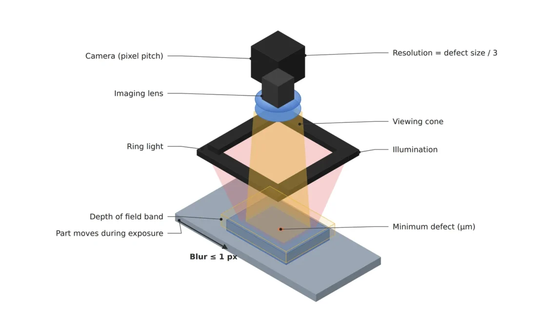
So before opening the algorithm I calculate three physical quantities: the size of one pixel, the distance the part moves during exposure, and the depth that stays in focus. If any one of the three falls short, nothing done afterward changes the result.

A crack must span three pixels to stay in the image

The first quantity is the length one pixel covers on the part, the object-side pixel resolution¹. Looking at a 40 mm field of view² with a camera 2,448 px wide gives 16.3 μm per pixel, and a 50 μm wide crack spans 3.06 pixels. My rule is that the finest defect spans at least three pixels, so this combination barely sits on the line.

Three pixels are needed because of how a crack overlaps the pixel boundaries. If the crack is one pixel wide, the moment it straddles a boundary its brightness difference splits in half over two pixels and sinks into the background, so the same crack shows or vanishes depending on where it lies. With three pixels, at least one pixel is filled by the crack and contrast remains wherever it falls. When the urge comes to widen the view, you have to calculate along with it that the pixels grow and the crack drops below three pixels. Viewing the same 40 mm with a camera 1,920 px wide makes each pixel 20.8 μm and drops the crack to 2.4 pixels, below the rule. A pixel count one step lower, chosen to save on the camera, ends up deciding whether the crack is found.

During a 1 ms exposure the part travels 0.5 mm

The second quantity is motion during exposure. If the part moves while the shutter is open, the image drags by that distance as motion blur³, and the motion equals speed times the exposure time⁴. A part passing at 500 mm per second shot for 1 ms moves 0.5 mm, which is 30.6 pixels. A crack three pixels wide gets rubbed along 30 pixels, and only a faint smudge is left in the image.

To hold the smear to half a pixel, 8.2 μm, the exposure must be 16.3 μs or shorter. Cutting from 1 ms to 16.3 μs reduces the incoming light to one sixty-first. Packing the pixels more densely does not help either. Smaller pixels only spread the same 0.5 mm over more of them, so the higher the resolution, the shorter the exposure has to be.

This is why lighting sets the ceiling of performance on a fast line. Unless light is added in step with the shorter exposure, the image darkens and the small brightness difference of the crack falls below the sensor noise. Software can read the remaining contrast more precisely, but it cannot create the information that disappeared while the shutter was open.

The depth in focus must cover the seating height variation

The third quantity is depth of field⁵. A part does not sit in the fixture at exactly the same height every time, so assuming the seating height varies by ±0.5 mm, focus must hold over 1.0 mm front to back. At a magnification of 0.21, an 8.45 mm wide sensor viewing 40 mm, a 25 mm lens sits about 143 mm from the part measured from the lens center, and with the circle of confusion⁶ set to two pixels, 6.9 μm, the depth of field at f/2.8 is 1.05 mm. That leaves almost no margin.

Stopping the f-number⁷ down one stop to f/4 widens the depth of field to 1.50 mm, but the incoming light halves again. Stop down further and diffraction⁸ gets in the way. At f/4 the diffraction blur spot is 6.5 μm across, 1.9 pixels, and at f/8 it reaches 13.0 μm, 3.8 pixels, larger than the three-pixel crack. If it were my setup, I would stop at f/4.

All three quantities converge on the amount of light

Line up the three numbers and a common opponent appears. Narrowing the view to protect resolution means more cameras or pixels, cutting the exposure to 16.3 μs to stop the smear leaves one sixty-first of the light, and stopping down to f/4 for depth halves it again. Getting the brightness of a continuous light shot at 1 ms and f/2.8 at 16.3 μs and f/4 takes about 125 times the instantaneous illuminance⁹, and that number is the starting point for choosing strobe lighting¹⁰. It also means that changing only the exposure and aperture while keeping the continuous light as it is records the same scene at one 125th of the brightness.

The design order follows the same calculation. The defect size gives the pixel size, the pixel size gives the view and pixel count, the speed gives the exposure, and the exposure gives the light.

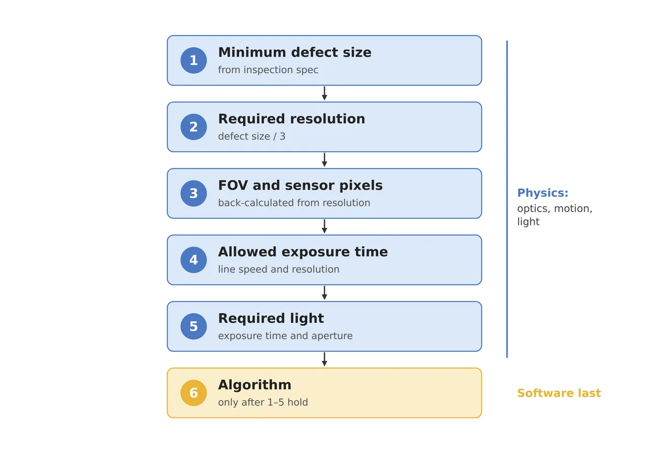
The algorithm sits at the bottom of the six steps in the figure because only once the five boxes above it are fixed does an image exist for the algorithm parameters to rely on. Walk the order backward and later you cannot even tell which part to fix.

Quantity	① Minimum defect size	② Optical setup · WD	③ Algorithm parameters · in plain words
Pixel resolution	50 μm crack = 3.06 px (16.3 μm/px)	2,448 px wide with 3.45 μm pixels, 25 mm lens, 40 mm view, WD about 143 mm (from the lens center)	Minimum crack candidate width 3 px. Widen the view and recalculate this value first
Motion during exposure	Smear of half a pixel = 8.2 μm or less	500 mm/s, exposure 16.3 μs or shorter, strobe lighting (about 125 times the instantaneous illuminance of continuous light)	Measure the edge smear on the raw image and flag an image-quality warning before judgment for frames beyond half a pixel
Depth of field	Crack keeps 3 px even at ±0.5 mm seating height (assumed)	f/4, depth of field 1.50 mm, diffraction blur 1.9 px (3.8 px at f/8)	Drop frames whose focus score is below the reference from judgment and signal a retake

If any one of the three rows has a gap, the numbers in ③ lose their meaning, because the algorithm parameters assume an image in which the first two columns are filled. On the other hand, if defects are larger than ten pixels and the part is shot while standing still, the physics already has room to spare, and working on the algorithm and training data is the faster path. Whether the crack contrast on a matte housing comes out as large as this calculation cannot be guaranteed before a sample test.

If a person cannot see it, the algorithm has nothing either

When an inspection goes badly, there is one question to ask: can a person see the defect when looking at this raw image at 100 % scale? Before opening the algorithm window, I check by eye on the raw image whether the crack spans three pixels or more, whether the edge smear stays within half a pixel, and whether focus holds to the edge of the frame. If any of these is off, the place to fix is the optics and lighting. Only when all three answers are yes does the turn come to touch the threshold.

When a machine vision engineer gets these numbers right at the setup stage, commissioning spends less time repeating retraining. On the purchase order, a strobe light and controller are a cost added to the camera, but saving on them turns the whole inspection machine into a device that cannot deliver its numbers. This article explains technology and is not investment advice. See our Disclaimer.

Field Note

For a new setup with this housing, I shoot one crack sample standing still, then pass the same sample at 500 mm per second and compare two frames side by side, one at a 16 μs exposure and one at 50 μs. At 50 μs the smear becomes 1.5 pixels, so watching whether the crack edge visibly dulls tells me whether the half-pixel rule holds for this material too. I also keep one frame each with a 0.5 mm shim under the fixture to change the height, and check whether focus at the edge of the frame holds at f/4.

Field Checkpoints

Once the still frame and the moving frame sit side by side, you can answer the questions below with numbers.

• Is a WD of about 143 mm (25 mm lens, from the lens center) secured even after adding the strobe light and fixture? (whether there is room for the light beside the lens)
• Does the finest crack span three pixels or more? (for a 50 μm crack, 16.7 μm per pixel or less)
• Is the smear calculated from the exposure time and speed half a pixel or less? (16.3 μs or shorter at 500 mm/s)
• Does the seating height variation fit inside the depth of field? (1.50 mm at f/4, 1.05 mm at f/2.8)
• Can the strobe light deliver about 125 times the instantaneous illuminance of the continuous light? (whether you check it in the light controller spec sheet)
• Can a person see the crack when looking at the raw image at 100 % scale? (if not, whether you go back to the optics)

Frequently Asked Questions

Would more camera pixels solve all three problems at once?

More pixels improve resolution, but as each pixel gets smaller over the same view, the smear during exposure spans more pixels and the exposure has to shrink further. Smaller pixels also make diffraction blur relatively larger, leaving less room to stop down. It is more accurate to treat the pixel count as a variable that forces all three quantities to be recalculated.

Would an AI model find the crack even in a blurry image?

A model learns the patterns left in the image, so in an image where the smear stays within half a pixel and the crack spans three pixels, it finds cracks more steadily than a person. In an image where the crack is rubbed along 30 pixels, as with a 1 ms exposure, no information remains to tell a crack from a smudge, and the judgment wavers however many training pictures you add. A model can only show its skill inside the image the optics hand over.

Glossary

• [1] Object-side pixel resolution object-side pixel resolution
  The length one pixel covers on the part. It is the view divided by the horizontal pixel count, written in μm/px. ↩
• [2] Field of view field of view, FOV
  The area on the part that one camera frame covers. ↩
• [3] Motion blur motion blur
  The image dragging and smearing in the direction of motion because the object moves during exposure. ↩
• [4] Exposure time exposure time
  The time the sensor collects light. The shorter it is, the less smear and the darker the image. ↩
• [5] Depth of field depth of field, DOF
  The depth over which things stay sharp in front of and behind the distance you focus on. It widens as you stop down. ↩
• [6] Circle of confusion circle of confusion
  The diameter up to which a point blurred by defocus is still counted as sharp. The text uses two pixels, 6.9 μm. ↩
• [7] F-number f-number
  The focal length divided by the lens opening diameter. Stopping down one step from f/2.8 to f/4 roughly halves the incoming light. ↩
• [8] Diffraction diffraction
  Light spreading as it passes a narrow opening. The more you stop down, the larger a point blurs, softening the edges of fine defects. ↩
• [9] Illuminance illuminance
  The amount of light reaching a surface, in lx. Shortening the exposure requires raising the illuminance by the same factor for the same brightness. ↩
• [10] Strobe lighting strobe lighting
  Lighting that fires short and strong only at the moment of exposure. It can reach a much higher instantaneous brightness than continuous lighting. ↩

References

• Formulas: pixel size = view ÷ horizontal pixel count; motion during exposure = speed × exposure time; allowed exposure = 0.5 × pixel size ÷ speed; magnification m = sensor width ÷ view; lens-center-to-object distance u = f × (1 + m) ÷ m; depth of field ≈ 2 × N × c × (1 + m) ÷ m²; diffraction blur diameter ≈ 2.44 × λ × N × (1 + m) (λ = 0.55 μm); light ratio = exposure time ratio × (f-number ratio)²
• Assumed values: a 2,448 × 2,048 px camera with 3.45 μm pixels, a 25 mm lens, a seating height of ±0.5 mm, and a reference continuous light at 1 ms and f/2.8 are assumptions for the worked example

Related reading — How to Calculate Machine-Vision Lens Focal Length · A Machine Vision Lens Calculator That Catches the FOV Error a Shortcut Formula Misses · Reserve Room for Vision Cameras and Lighting at the Mechanical Design Stage