Shorter Exposure Means a Darker Image, So How Do You Freeze Motion? — Suppressing Motion Blur on the Move with Strobe Overdrive

LIGHTING / STROBE

At inspection sites where moving targets must be imaged without stopping them, the same conversation repeats. The image is blurry, so shorten the exposure; shortening the exposure makes it dark, so raise the gain; raising the gain makes noise look like defects. In the end the setup settles on a compromise that gives up one side between exposure time and brightness, and that compromise collapses again as soon as the line speed rises a little.

Left unaddressed, the cost appears first at the smallest defects. Motion blur stretches the outline of a defect in the direction of travel and dilutes its contrast. When the blur width approaches the defect size, an 80 µm-class dent on a pin tip or a silkscreen smear blends into the background and passes. Conversely, if the threshold is set lower, normal edges smeared by blur pour out as over-detections. Either way, the inspection result becomes a value that wobbles along with the line speed.

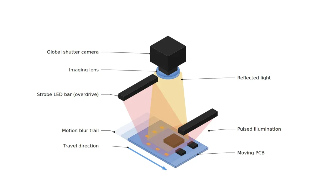
The solution is to replace the shutter with the time the illumination is on, not with the camera exposure. If the illumination is turned on briefly as a pulse a few µs wide, then even if the camera exposure window is longer, the time in which an image actually forms is only the pulse width. The light lost to the shorter time is made up by overdrive, which drives the LED momentarily above its rated current. The starting point of the design is a one-line calculation: blur px = speed × pulse width ÷ pixel resolution.

In imaging on the move, the shutter is not the camera but the width of the illumination pulse.

1. Set the Blur Tolerance in px First

Point. Strobe design starts not with choosing a pulse width but with setting the allowable blur in px first.

Reason. The length of motion blur is the product of the target’s travel speed and the time light comes in. Dividing this length by the pixel resolution (µm/px) gives how many px it smears across the image. If the blur is 0.5 px or less, the edge slope is almost indistinguishable from the stationary state; beyond 1 px, the edge width widens noticeably; and as it approaches the px occupied by the smallest defect, detection itself becomes unstable. Therefore, once the allowable blur is set first, the required pulse width is determined by back-calculation.

Example. Assume a travel speed of 1,000 mm/s, a FOV of 60 mm, and a sensor 2448 px wide. The pixel resolution is 60 mm ÷ 2448 px ≈ 24.5 µm/px. With continuous illumination and a 100 µs exposure, the blur is 1,000 mm/s × 100 µs = 100 µm, about 4.1 px. Since the minimum defect of 80 µm is about 3.3 px, the blur is longer than the defect. If the allowable blur is set at 0.5 px (about 12.3 µm), the pulse width must be 12.3 µs or less, and choosing 10 µs with some margin gives a blur of 10 µm, about 0.41 px.

Point. Write on the first line of the specification sheet not “it is blurry, so shorten the exposure” but “how many px of blur is allowed”. Control of the travel speed itself requires a separate review, but the speed value is an essential input to this calculation.

2. Overdrive — The Conditions for Raising Current as Much as the Time Is Shortened

Point. Shortening the pulse width to 10 µs leaves the light insufficient, and overdrive is the method of filling this shortfall with current. However, what sets the limit is often the peak condition of a single pulse rather than the average duty ratio.

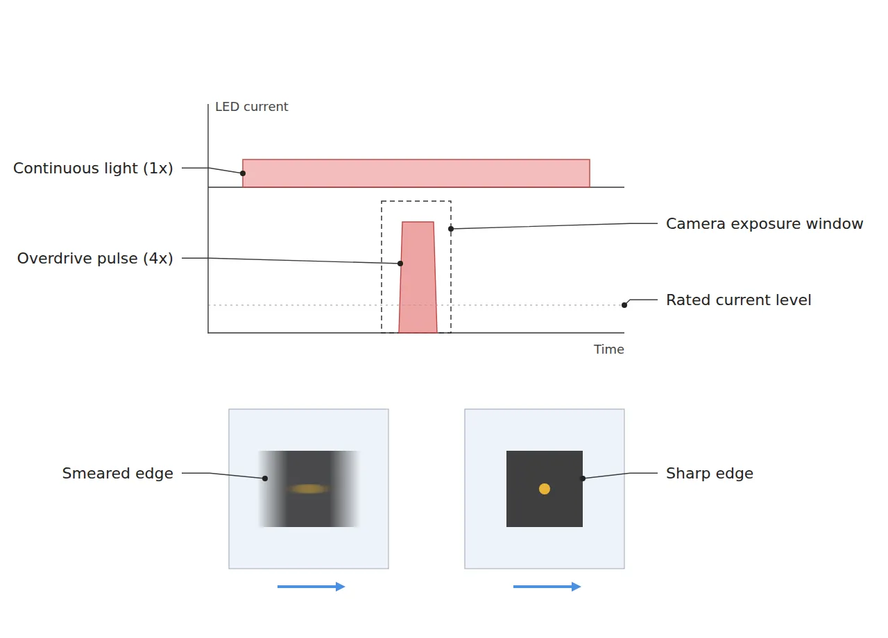
Reason. The thermal limit of LED illumination is usually explained by average power, that is, peak power × duty ratio. But if the pulse is only a few µs long and the imaging period is tens of ms, the duty ratio becomes very small and average heating is hardly an issue. The constraints then move to the peak current the LED chip and driver can withstand, the junction temperature rise during a single pulse, and the current rise time of the driver. In addition, LED light output is not directly proportional to current, and its rate of increase slows in the high-current region, so four times the current does not guarantee four times the light.

Example. With the imaging rate set at 20 fps (one frame every 50 mm of travel, 10 mm overlap with a 60 mm FOV), the duty ratio of a 10 µs pulse is 10 µs × 20 = 200 µs/s, that is, 0.02%. Even overdriven at four times the rated current, the average heating falls far short of even 1% of rated continuous operation. On the other hand, if the driver current rise time is 1 µs, 10% of a 10 µs pulse is spent in the rise section, so the shorter the pulse, the larger the proportion of effective light lost. The combination of allowable current and pulse width must be confirmed with the illumination manufacturer’s pulse rating data.

Point. An overdrive review sheet must list, side by side with the duty ratio, the three items peak current, maximum pulse width and driver rise time. Judging it safe by looking only at the duty ratio comes back as a slow failure called chip degradation.

3. Closing the Pulse Width vs. Light Trade-Off on the Optical Side

Point. In most cases overdrive alone does not fully restore the light, and the remaining shortfall should be sought first in the aperture and illumination layout rather than in gain.

Reason. The light energy accumulated in one frame is roughly proportional to light output × illumination on-time. Changing a configuration that exposed for 100 µs with continuous illumination at 1× to 10 µs with 4× overdrive drops the energy to (4 × 10) ÷ (1 × 100) = 0.4×, that is, 40%. In practice it may be lower because of LED efficiency droop. Filling the shortfall with gain amplifies signal and noise together, so the contrast-to-noise ratio does not improve. Reversing the blur of a long exposure with software deblurring has the same noise amplification problem and cannot fully cover a shortfall in the hardware setup.

Example. Opening the aperture one stop from F/8 to F/5.6 roughly doubles the collected light, restoring the energy from 0.4 to about 0.8×. The depth of field narrows at this point, so it must also be checked whether the height variation of the target stays within the depth. The remaining factor of about 1.25× is secured by shortening the illumination working distance or adding illumination units, and gain is left as the last resort. The camera exposure window is set to 20 µs to enclose the 10 µs pulse with trigger jitter margin, and a light-shielding hood is fitted so that ambient light does not contribute within this short window. The light required on surfaces that mix in diffuse reflection, such as the glossy metal parts of a connector, cannot be confirmed before sample testing.

Point. Always calculate the sharpness gained by shortening the pulse width and the light lost in return as an energy ratio within the same table. Only then is it decided at the design stage whether the shortfall closes with the aperture or requires additional illumination.

The price of cutting blur to one tenth is a 60% loss of light energy, and where to make up that loss is the body of strobe design.

4. Core Framework — Matching Table

Category	Item	Specification / Parameter	Basis & Notes
① Minimum defect size	Dent on connector pin tip	80 µm or more	Design assumption. Occupies about 3.3 px at 24.5 µm/px
① Minimum defect size	PCB silkscreen print smear	100 µm or more	Design assumption. Occupies about 4.1 px
① Minimum defect size	Residual solder ball	Diameter 120 µm or more	Design assumption. Occupies about 4.9 px
② Optical setup	Illumination	Two LED bar lights, strobe pulse 10 µs, 4× rated overdrive	Design assumption. Confirm allowable current and pulse width with the manufacturer’s pulse rating
② Optical setup	Synchronization	Imaging at 20 fps, duty ratio 0.02%, trigger jitter 1 µs or less	Jitter 1 µs × 1,000 mm/s = 1 µm (about 0.04 px, calculated value)
② Optical setup	Lens	Focal length 16 mm, F/5.6	Magnification about 0.141×, calculated object distance about 130 mm
② Optical setup	WD (working distance)	110 mm or more must be secured	Measured from the lens front end. Verify by measurement including interference from bar lights and hood
② Optical setup	Sensor & FOV	Global shutter 2448 × 2048 px / FOV 60 mm × 50 mm	60 ÷ 2448 ≈ 24.5 µm/px (calculated value)
③ Algorithm	Blur tolerance	0.5 px or less (1,000 mm/s × 10 µs = 10 µm ≈ 0.41 px)	About 4.1 px with continuous illumination and 100 µs exposure (comparative calculated value)
③ Algorithm	Blur verification	Measure edge 10–90% width while moving, increase over stationary 0.5 px or less	Measured by passing a calibration pattern at actual speed
③ Algorithm	Brightness normalization	Per-frame gain correction from the mean brightness of a reference plate, with a gain upper limit	For tracking pulse-to-pulse light variation
③ Algorithm	Defect judgment	Difference from background > 3σ, minimum area 6 px or more	Based on an 80 µm defect area of about 3.3 × 3.3 px = about 10.7 px

Table implication. At 24.5 µm/px, the minimum defect of 80 µm occupies about 3.3 px, barely exceeding the detection floor. The 4.1 px blur of continuous illumination at 100 µs is larger than this defect and erases it in principle, whereas the 0.41 px blur of a 10 µs pulse is only about one eighth of the px the defect occupies. The price, light energy at 40%, recovers to 80% with one aperture stop (about 2×), so whether the remaining shortfall can be closed by the illumination layout decides the success of this configuration.

5. When the Opposite Approach Wins

• Indexed processes in which the target stops at the moment of imaging: Blur is absent in principle, so continuous illumination and a long exposure are favorable in both light and stability, and chip stress from overdrive can be avoided.
• Configurations with slow travel or coarse pixel resolution: If speed × exposure calculates to 0.5 px or less, the complexity of a strobe (sync wiring, driver) brings no benefit.
• High-speed imaging with a very short frame period: When the duty ratio grows and average heating nears its limit, the overdrive factor must be lowered, so a structure that keeps the illumination on continuously, as in line scan, may be better.

The required overdrive factor varies with surface reflectance and the degree of LED efficiency droop, so the actual light margin cannot be confirmed before sample testing.

Field Note

When inspecting connector pin tips on a high-speed assembly line, I once held out by shortening the exposure and raising the gain before finally switching to a strobe. At first I thought it would be enough to shorten the pulse width to 10 µs, but even with overdrive it did not get as bright as calculated, and only after opening the aperture one stop and moving the bar lights closer did the light add up. When I measured the edge width of a calibration pattern on the move, the increase over the stationary state was within 0.5 px, and only then did I set the threshold again. The duty ratio had a large margin, but I learned that the driver rise time took up a considerable part of the pulse only after capturing the waveform. Results can differ when illumination and surface conditions change, so I now put the waveform check at the first step of setup.

Field Checkpoints

• Is a WD of 110 mm or more secured by actual measurement? — Check together whether the bar lights and light-shielding hood fit between the lens front end and the target.
• Have the surface material and reflectance of the target been checked first? — Metal pins and solder mask need different amounts of light even under the same pulse.
• Has the pulse width been back-calculated from the allowable blur (px) and travel speed and written in the specification sheet?
• Have the peak current, maximum pulse width and driver rise time been confirmed against the manufacturer’s rating together with the duty ratio?
• Has the illumination current waveform actually been measured to confirm the effective pulse width? — The rise section is lost light.
• After changing the aperture, does the depth of field cover the height variation of the target?