When Light Runs Short, a SPAD Sensor Counts Photons Instead of Extending Exposure

OPTICS

Counting photons in place of a longer exposure removes read noise, but a 256-pixel sensor shrinks the field to about 4 mm, and time gating cuts only light that has wandered more than 20 mm inside the resin.

Using a fine crack under a translucent resin cover as the example, I compared the noise, field of view and gate timing of a standard CMOS sensor and a SPAD sensor in the same numbers.

About 15 min read

When light runs short, you lengthen the exposure, raise the gain if that is not enough, and finally switch the lighting one step brighter. It is a plausible order and usually works. Where the signal has dropped to a few photons per pixel, though, as with a 30 μm crack under a translucent resin cover, all three stall. Exposure grows motion blur, gain grows read noise¹ along with the signal, and brighter lighting also brightens the light scattered inside the cover, which covers the edges of the crack.

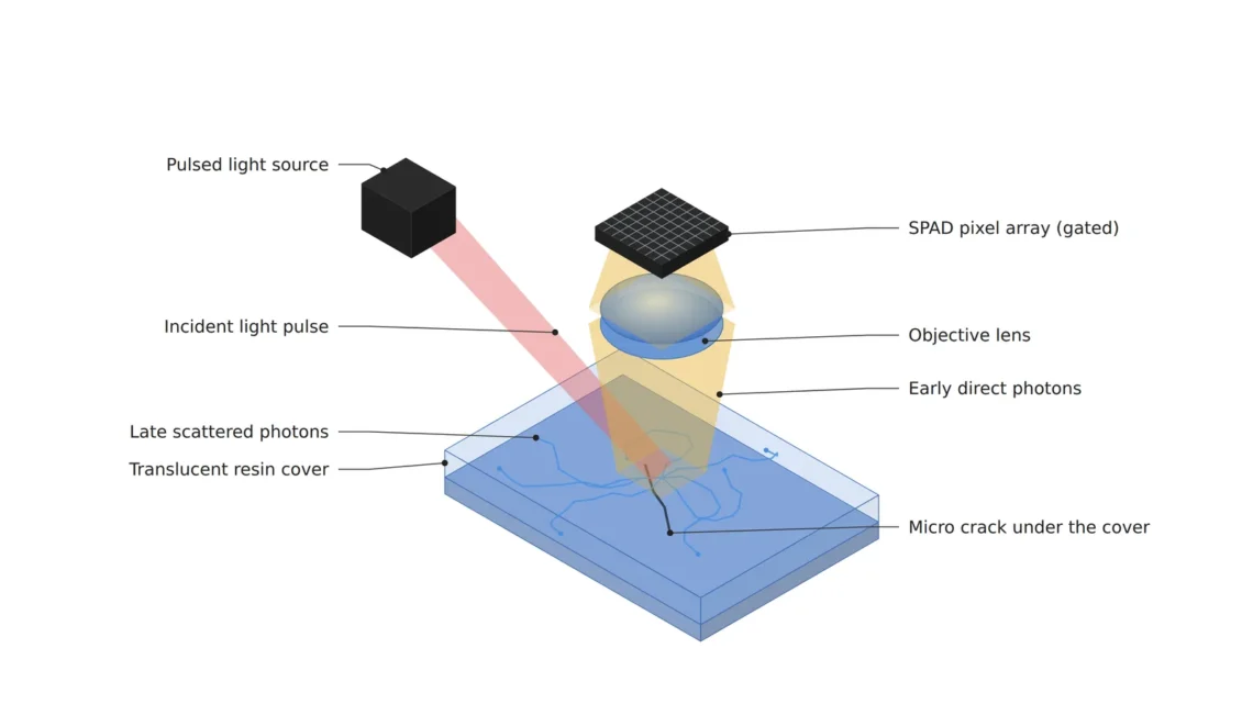
The cover is a translucent resin that lets some light through and scatters it inside, so light coming straight back from the surface and light that wandered inside before emerging mix in the same pixel. When the scattered light lifts the background into a haze, the contrast at the crack edges collapses, and the crack passes inspection and comes back as a fracture only after assembly.

A single-photon avalanche diode (SPAD)² sensor attacks this problem along another axis. It counts each photon as a digital pulse, which removes read noise, and with time gating³, which counts only photons arriving in a set time window synchronized to pulsed lighting, it can discard scattered light that arrives late. What I want to work out is how much those two gain in numbers, and what they give up in return.

Longer exposure brings more blur with it

Lengthening the exposure gathers more photons, but if the part moves in the meantime, the gathered photons smear into neighboring pixels. At 16.7 μm/px, which puts a 50 μm particle on three pixels, a part moving at 10 mm per second (assumed) limits the exposure to 1.67 ms to keep the blur within one pixel. Double the exposure and the photons double, and so does the blur, to two pixels.

Another way around the blur is to shoot many short frames and add them up. On a standard CMOS sensor this carries a price, because read noise is added once every time a frame is read. Assume 100 photons reach the pixel and calculate with a quantum efficiency of 0.6 and 2 e⁻ of read noise: one long exposure gives a signal-to-noise ratio of 7.5, while splitting the same photons over 30 frames and adding them drops it to 4.5. The noise piled up over 30 reads grows larger than the shot noise⁴ from the 60 e⁻ of signal.

A standard CMOS sensor stands at a fork: shoot long and it blurs, split the shot and the noise piles up. A counter with no read noise steps around that fork.

Counting without read noise lets short frames add up freely

A SPAD pixel puts out a digital pulse from the avalanche breakdown triggered by a single photon, and what it measures is the number of pulses more than charge. No analog noise is added in reading, so thirty 1 ms frames added together have the same statistics as one 30 ms frame. The photon detection efficiency⁵, the rate at which photons become pulses, tends to be lower than the quantum efficiency of standard CMOS, though; take it as 0.3 and the same 100 photons give a signal-to-noise ratio of 5.5.

Set the three numbers side by side and the place where SPAD wins can be calculated. Under the condition of splitting into 30 frames, SPAD beats standard CMOS when fewer than 6.7 photons reach a pixel per frame, and with a detection efficiency of 0.5 that boundary rises to 33. For a stationary part that can be shot in one long exposure, the 7.5 of standard CMOS is hard to beat. My judgment is that the gain of SPAD lies less in sensitivity than in adding short, blur-free frames with no noise penalty.

In place of read noise, a SPAD has pulses that occur even without light, the dark count⁶. Gating reduces these as well: fire pulses at 20 MHz and open the gate for only 1 ns each time, and the gate is open 2 % of the time, so the dark count drops to one fiftieth. With plenty of light, on the other hand, SPAD is the first to choke. A pixel that has just fired cannot take the next photon for a moment, so even an average of 0.1 photons per pulse causes pile-up⁷ that misses 4.8 %, and at 20 MHz about 1.9 million counts per second is the limit for 5 % loss.

The three numbers show from both sides that SPAD is a sensor tuned for darkness. It wins when photons per frame are in the single digits, and it loses counts once photons per pulse pass 0.1. That makes it hard to combine with the fix of brighter lighting.

With 256 pixels the field of view is 4.27 mm

There is news on the sensor side as well. On September 10, 2026, Singular Photonics of Edinburgh announced Litavis, a SPAD image sensor. According to the company, it delivers continuous 256 × 256 px photon-counting images while recording picosecond-resolution photon timing on a 64 × 64 macropixel⁸ grid, running intensity, timing and histogram modes at the same time. Pixel pitch, detection efficiency and dark count are not given in that announcement, so every value put into the calculations above is an assumption.

Resolution sets the field of view directly. Putting a 50 μm particle on three pixels means 16.7 μm/px, so 256 pixels see 4.27 mm, and putting a 30 μm crack on three pixels means 10 μm/px and a field shrunk to 2.56 mm. For a 200 μm long scratch it can widen to 17.1 mm. Covering a 40 × 40 mm cover with a 4.27 mm field and 10 % overlap takes 11 × 11, or 121, tiles, so this sensor suits a second look at suspect spots better than a camera that sweeps the whole part.

The timing grid is coarser still. A 64 × 64 macropixel grid bundles 4 × 4 pixels into one cell, so at 16.7 μm/px timing information comes only every 66.7 μm. Separating scattered light by arrival time happens on a grid coarser than a single particle. The lens and WD⁹ depend on the pixel pitch; take the pitch as 10 μm (assumed) and the magnification is 0.6, so a 50 mm lens gives a WD of about 133 mm and a 75 mm lens about 200 mm. Leaving room for the pulsed light source and its synchronization wiring in front of the lens, I would choose the 75 mm.

What 100 ps separates is 20 mm of path inside the resin

The gain from time gating is calculated with the speed of light. In air, light travels 0.3 mm per picosecond, and inside resin with a refractive index of 1.5 it travels 0.2 mm. Light that goes to the back face of a 2 mm cover and returns arrives 20 ps after the front-surface reflection. Taking the time resolution, pulse width plus the sensor’s timing jitter¹⁰, as 100 ps (assumed), the only light a gate can separate is light that wandered more than 20 mm farther inside the resin than the front reflection. The figure is a concept diagram of this situation drawn by photon arrival time.

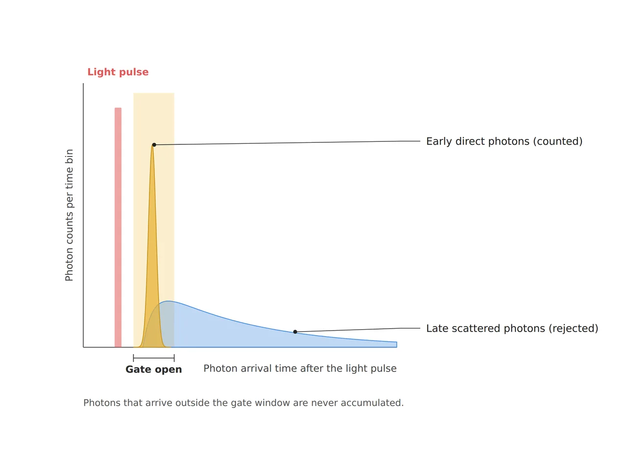
The sharp peak of direct reflection is counted inside the gate, and the part of the broad scattered tail that arrives after the gate is thrown away. The trouble is the front of the tail. Light that wanders only a few millimeters inside the cover arrives within 100 ps of the direct reflection and enters the gate along with it, and much of the haze around a crack may come from such short paths. Cutting that light too would take the time resolution down to around 20 ps, a condition that requires both pulse width and jitter to shrink that far and narrows the equipment choice sharply.

So I see time gating as a tool for trimming the late tail of scattering more than for erasing scattering. The gain is large for thick translucent parts where light wanders centimeters inside the resin, or for separating light that arrives several nanoseconds late, such as fluorescence, and it may be small for a crack on the surface of a 2 mm cover. Its size depends on the scattering properties and thickness of the resin and cannot be guaranteed before a sample test.

Photons have to be counted on the chip for the data path to hold

Send every photon off the chip with its arrival time and the data path gives way first. Even if each of the 256 × 256 pixels counts only 1,000 photons per second, tagging each photon with a 16-bit time comes to 1.05 Gbit per second, more than a single Gigabit Ethernet link, and at 100,000 per second it is 105 Gbit. Folding the same information into a 32-bin arrival-time histogram¹¹ for each of the 64 × 64 macropixels and sending it 30 times per second brings it down to 63 Mbit.

This calculation is where the Singular Photonics description, processing photon events directly on the chip to sharply cut the raw data sent outside, comes in. A SPAD evaluation is therefore an optical review and a data-path review at once. Narrowing the gate lowers the counts and the bandwidth, but reaching the same statistics takes more stacked frames, so the inspection time can grow. Techniques that handle this trade in circuitry also appear in patents.

Patent	Title	Assignee	Priority · granted
US 10,620,300 B2	SPAD array with gated histogram construction	Apple Inc.	2015-08-20 · 2020-04-14
US 10,801,886 B2	SPAD detector having modulated sensitivity	Apple Inc.	2017-01-25 · 2020-10-13

The first patent attaches a processing circuit to each pixel to control the time window in which it can take photons, sweeps that window first to find each pixel’s position, then fixes it to build a fine arrival-time histogram. The second varies SPAD sensitivity within each light-pulse interval, across the whole array or by section, with methods such as histogram bins of unequal time width or changing the quenching transistor’s signals to alter the recharge time. Implementing a gate-delay sweep in-house to get the time distribution calls for a separate review of the claim scope.

Low-light setup table for one crack

Gathering the numbers into one table shows that the specification for low-light inspection is written in photon counts and time more than in brightness. The first row also records that the crack, the particle and the scratch each demand a different field of view.

Item	Value	Condition · basis	In plain words
① Minimum defect size (μm)	Crack 30 μm wide, particle 50 μm across, scratch 200 μm long	10 · 16.7 · 66.7 μm/px for three pixels, 256-pixel field of 2.56 · 4.27 · 17.1 mm	Each defect sets its own field of view
② Lighting	Pulsed source (20 MHz, synchronized to the gate), 1 ns gate, 0.1 photons per pulse or fewer	Time resolution 100 ps (pulse width + jitter, assumed) = 20 mm in resin. Pile-up 4.8 %, gate duty 2 %	Only late light can be thrown away
② Sensor · lens · WD	SPAD 256 × 256 px, timing on 64 × 64 macropixels (Litavis published specification), 10 μm pixel pitch assumed	75 mm lens, 0.6 magnification, WD of about 200 mm must be secured (thin-lens approximation), recalculated once the pitch is confirmed	The lens is set only once the pixel pitch is known
③ Algorithm parameters	30 frames of 1 ms accumulated, time distribution from a gate-delay sweep, dark-count map subtracted (taken at operating temperature)	Threshold 3σ (√N based, re-estimated from 30 good parts), on-chip histogram output 63 Mbit/s	Shoot short and add without noise

The first cell to check in this table is the time resolution in ②. At 100 ps, light that wandered less than 20 mm in the resin cannot be separated, so for a crack in a 2 mm cover the gain from the gate may be smaller than the other cells suggest. The 2.56 mm field of view deserves the same weight. Covering a whole cover would take hundreds of repositioned shots, so I would bring this sensor in to take a second look at candidate spots found by an ordinary camera.

The opposite choice is the better one under some conditions. Under ordinary, ample lighting, SPAD chokes on pile-up first, so a standard CMOS global shutter wins on both resolution and price, and inspections that need several megapixels do not fit 256 × 256 px either. Opaque matte surfaces with almost no scattering have no light to cut by time, so angled lighting or polarization is more economical. Which way fits depends on the scattering time distribution of the material and cannot be guaranteed before a sample test.

Building the optics is the vision engineer’s job, but the time cells of this table have to be set together with whoever chooses the lighting driver and the sensor. How many picoseconds the assumed 100 ps of pulse width plus jitter actually turns out to be decides the gain from the gate. When comparing quotes, I recommend working out first that the tact time is set by how many times a field of a few millimeters has to be moved and shot, more than by the label of photon counting. This article explains technology and is not investment advice. See our Disclaimer.

Field Note

To bring SPAD into a low-light station, I would first sweep the gate delay in 100 ps steps on an actual cover, before setting the gate width, and see at how many picoseconds the direct-reflection peak and the scattered tail part ways. If the scattering crowds within 200 ps after the peak, I would treat the gain available from the gate as small and look at frame accumulation and other lighting angles together. I would retake the dark-count map at operating temperature and confirm from the count rate that photons per pulse stay at or below 0.1.

Field Checkpoints

Once the gate sweep and the dark-count map have been checked, go over the points below before finishing the setup.

• Is a WD of about 200 mm from lens to cover (75 mm lens, 10 μm pixel pitch assumed) actually available, clear of the pulsed source housing and synchronization wiring? (recalculated with the confirmed pixel pitch)
• Is the field of view small enough to put the target defect on three pixels or more? (2.56 mm for a 30 μm crack, 4.27 mm for a 50 μm particle)
• Has the number of photons per pixel per frame been calculated from light output, exposure and aperture? (lux values alone say nothing about counting statistics)
• Has the time resolution, pulse width plus sensor jitter, been confirmed? (at 100 ps, light that wandered less than 20 mm in resin cannot be separated)
• Are photons per pulse below 0.1? (above that, pile-up loses counts)
• Was the dark-count correction map taken at operating temperature?
• Does the data leaving the chip fit within the link bandwidth? (raw events easily exceed 1 Gbit/s)

Frequently Asked Questions

Would raising the gain on standard CMOS give the same effect?

Gain amplifies the noise ahead of it along with the signal, so as long as the photon count stays the same it cannot pass the limit set by shot noise. All gain reduces is the share of noise added in the later conversion stage, and with 100 photons the ceiling on the signal-to-noise ratio is 7.7 at a quantum efficiency of 0.6. Where the exposure cannot be lengthened, the ways to raise the signal-to-noise ratio are lighting and brighter lenses that gather more photons, or a sensor that adds frames without read noise.

Does time gating require a laser?

The time a gate can separate cannot be shorter than the pulse width, so with an LED pulse a few nanoseconds wide only differences of hundreds of millimeters in resin can be separated. One nanosecond corresponds to 200 mm inside resin. Getting near 100 ps calls for a source such as a picosecond pulsed laser diode, and the eye-safety class and reflection shielding of that source need a separate review.

Glossary

• [1] Read noise read noise
  Noise added when the charge collected in a pixel is read as a voltage and turned into a number. It is added once every time a frame is read. ↩
• [2] SPAD single-photon avalanche diode
  A diode that triggers an avalanche breakdown and puts out a digital pulse when a single photon arrives. It measures light as a count of pulses. ↩
• [3] Time gating time gating
  Counting only the photons that arrive in a set time window after a lighting pulse. It filters out late scattered light by time. ↩
• [4] Shot noise shot noise
  Statistical fluctuation that comes from photons arriving one by one. With an average of N, the fluctuation is √N, so it shrinks only with more photons. ↩
• [5] Photon detection efficiency PDE
  The share of photons reaching a pixel that actually become pulses. It corresponds to the quantum efficiency of an ordinary sensor. ↩
• [6] Dark count dark count
  False pulses produced without light, by heat and other causes. They rise with temperature, so the correction map is taken at operating temperature. ↩
• [7] Pile-up pile-up
  Undercounting at high light levels because a pixel that has fired cannot take the next photon for a moment. Even 0.1 photons per pulse loses about 5 %. ↩
• [8] Macropixel macropixel
  A unit that bundles several pixels into one cell to process timing information together. Bundling 256 × 256 pixels into 64 × 64 makes each cell 4 × 4 pixels. ↩
• [9] WD working distance
  The distance from the lens to the surface being inspected. The value in the text uses a thin-lens approximation measured from the lens center. ↩
• [10] Timing jitter timing jitter
  How much the time a sensor records wobbles even for photons arriving at the same instant. Together with the pulse width, it sets the shortest time a gate can separate. ↩
• [11] Arrival-time histogram arrival-time histogram
  A distribution built by counting, in time bins, how many picoseconds after the pulse each photon arrived. Sending this distribution in place of every photon’s time cuts the data sharply. ↩

References

• Singular Photonics, Singular Photonics launches world-first SPAD-based image sensor (September 10, 2026; Litavis: 256 × 256 px photon-counting imaging, picosecond timing on a 64 × 64 macropixel grid, simultaneous intensity · timing · histogram modes)
• Apple Inc., US patent US10620300B2, SPAD array with gated histogram construction (priority and filing August 20, 2015; granted April 14, 2020)
• Apple Inc., US patent US10801886B2, SPAD detector having modulated sensitivity (priority January 25, 2017; filed January 24, 2018; granted October 13, 2020)
• Formulas: blur-limited exposure = pixel resolution ÷ speed, CMOS signal-to-noise = QE·N ÷ √(QE·N + k·σr²), SPAD signal-to-noise = √(PDE·N), crossover photons = PDE·σr² ÷ (QE·(QE − PDE)), pile-up loss = 1 − (1 − e^−μ) ÷ μ, gate duty = gate width × repetition rate, field of view = 256 × pixel resolution, WD ≈ f × (1 + 1/m), speed of light in resin = 0.2998 mm/ps ÷ 1.5, raw data = pixels × count rate × 16 bits

Related reading — Changing the Sensor Means Recalculating the Illumination · A Depth Camera’s Error Grows with the Square of Distance · In SWIR Imaging, Lighting and Aperture Keep the Defect Contrast