Why Edge AI Vision Fails on the Factory Floor

EDGE AI

Shrink a 20 MP image into a 640 px input and a 60 μm scratch becomes 0.35 pixel, so when edge AI inspection wobbles, check one number per symptom before retraining.

Splitting the symptoms of a server-validated model wobbling on the line into input size, quantization, heat, latency, bandwidth and input degradation, I calculated the number to measure first for each.

About 12 min read

Put an inspection model that passed validation on a server onto an edge device, and for a while it usually runs fine. The trouble starts a few weeks later, in the afternoon, or on the day one more camera is added. It shows up as slightly lower accuracy or an occasional late decision, so the cause gets searched for only inside the model.

Start with retraining before linking symptom to cause, and after weeks spent changing the model, the same symptom comes back. When the cause sits outside the model, in input size, heat, latency, bandwidth or lighting change, retraining fixes nothing, and meanwhile the smallest defects quietly slip out first.

The example line looks for 60 μm scratches on a part that mixes a matte molded housing with glossy metal terminals. The camera is 20 MP (5,472 × 3,648 px) and the pixel resolution¹ is 20 μm/px, so a scratch covers three pixels in the original image. The order I recommend is one number per symptom. Retraining does not start before that number has been looked at.

When only fine defects vanish, count pixels at the input

If overall accuracy drops by only 1 to 2 percentage points while one defect class disappears, the first suspects are input size and quantization. Neither shows up much in average metrics. So per-class recall² and the number of pixels the defect covers at the model input go on my first line. In both cases the server-side validation metrics barely move, so the problem shows only when the defect samples missed on the line are counted again class by class.

Shrink the whole 20 MP image into a 640 × 640 px input, and the width falls to one 8.55th, stretching the length each pixel covers from 20 μm to 171 μm. The 60 μm scratch that covered three pixels in the original shrinks to 0.35 pixel and disappears, blended with its neighbors during the shrink. It is not even one dot. With tiling³, which cuts the image at full resolution into 640 px pieces, one frame becomes 9 across and 6 down, 54 tiles, at the cost of 54 times as many inferences. How a lightweight model’s output stride⁴ drops a defect below one cell is calculated in the knowledge distillation article, and tile overlap and latency in the tiled inference article.

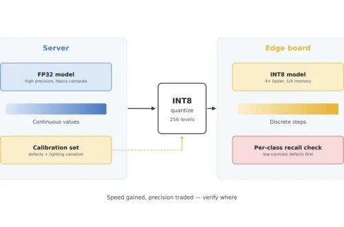
The third card is about quantization. INT8 quantization⁵ divides a tensor’s value range into 256 steps, and with the asymmetric scheme one step is range ÷ 255 wide. If a feature map spans 0 to 64 and the difference between scratch and background is 0.8, one step is 0.25 and the difference survives as 3.2 steps. So far, so good. But if blown-out highlights from the metal terminals get into the calibration⁶ images and widen the range to 0 to 256, one step becomes 1.0, and the 0.8 difference fills less than one step and can be merged into the same code as the background. Both numbers are assumptions for the calculation, but this structure explains the pattern in which only low-contrast classes lose recall.

So the number to check for this symptom is per-class recall before and after quantization. How many saturated highlights the calibration images contain belongs in the same check. Whether the quantization settings need changing continues in the INT8 quantization article and the server vs. edge accuracy article.

The hour it slows down points to the cause

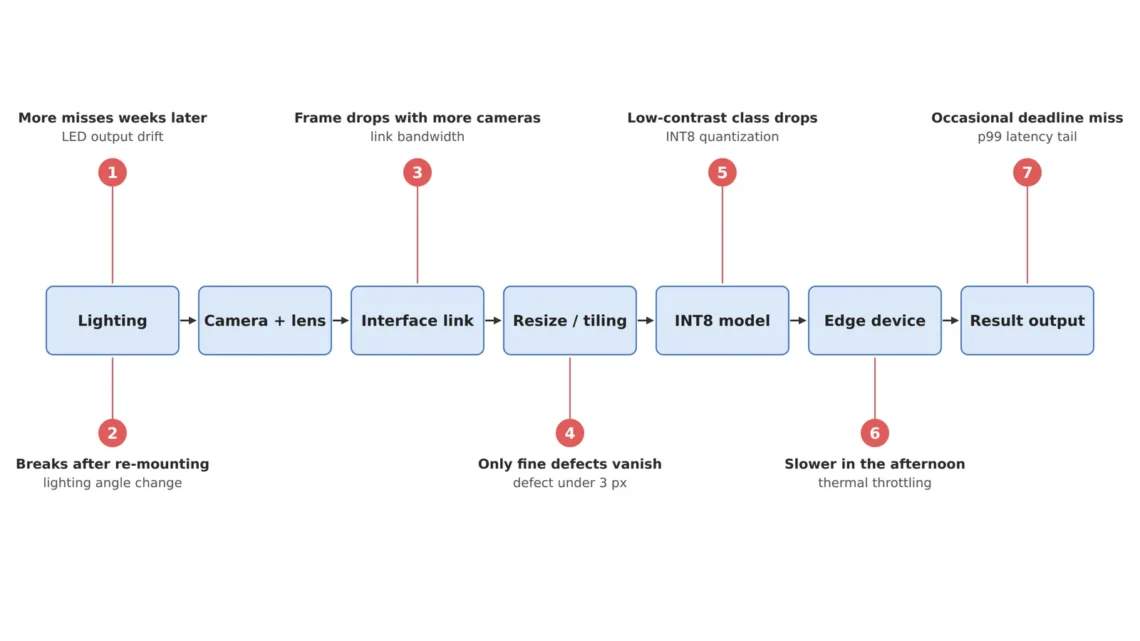
With speed problems, when it slows down points to the cause. The timetable is the clue. If it slows only in the afternoon, look at heat; if the average is fast but it is occasionally late, the latency tail; if frames drop after cameras are added, the interface. A fanless edge device lowers its clock as the temperature nears its limit, so inference time wobbles, and the cause appears nowhere in the model file. It only becomes visible when module temperature and inference time are logged on the same time axis; thermal design is calculated separately in the thermal design article.

Decision latency is the sum from trigger to output more than one inference stage, and it should be read as p99 latency⁷ more than as an average. On a line where two parts pass every second, if 1 in 1,000 misses the deadline, 57.6 parts in 8 hours do not get a verdict in time. Even with average inference at half the deadline, this number does not shrink. How to split it by stage is in the p99 latency budget article.

If frames start dropping on the day cameras are added, calculate the link first. Receiving 20 MP 8-bit images at 2 per second takes 39.9 MB/s per camera, and two cameras take 79.8 MB/s, within the roughly 115 MB/s assumed as the effective bandwidth⁸ of 1GigE. Hang a third camera on the same link, and it overflows at 119.8 MB/s. At that point I would log the real received MB/s per camera before shrinking the model. Options for widening or splitting the link are in the interface bandwidth article and the GigE Vision RDMA article.

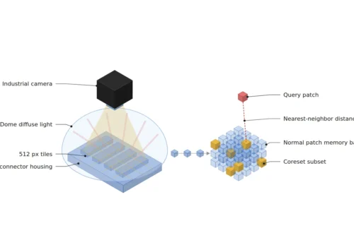
If the anomaly detection model stores normal features in a memory bank⁹ and compares against it, memory shortage or slow search appears as a separate symptom. The numbers to check then are latency and overdetection by coreset ratio, and that trade-off is calculated in the memory-bank anomaly detection article. A smaller bank searches faster but holds less normal variation and can raise overdetection, so the two numbers are weighed in the same table.

False calls weeks later mean the input changed

When performance changes slowly without any change to the model, the input has changed. Lens contamination, lighting degradation and focus drift leave traces in input statistics such as mean brightness and sharpness before they show in accuracy. Compute those two numbers every frame and plot the trend, and the cause can be seen moving before recall drops (input drift monitoring article).

Declining LED output moves toward missed detection first, with no alarm. In an inspection that catches a defect glowing at gray level 200 on a background of 120 with an absolute threshold of 170, the moment light output falls by 15% the defect drops to 170 and touches the threshold, and below that it is missed. A 15% drop is enough. Judged by the ratio to the background, the defect stays at 200 ÷ 120 = 1.67 times, above a threshold ratio of 1.42. As long as the light dims evenly, the ratio does not move. Degradation rates and recalibration intervals are in the LED degradation article.

A model that collapses after the light bracket is retightened has failed to learn a change in lighting angle that brightness augmentation cannot imitate. The number to check here is recall per lighting condition, and a capture plan that holds out one azimuth to measure how far recall drops under unseen lighting is in the lighting augmentation limits article. Retraining starts when these two numbers point to the model as the cause.

Nine symptom lines on one page

Lay out the numbers above in symptom order, and they become one page of troubleshooting map. The figure links symptom, first number to check and likely cause in three columns, and the table below widens the same map to include checking WD and resolution on the optical side.

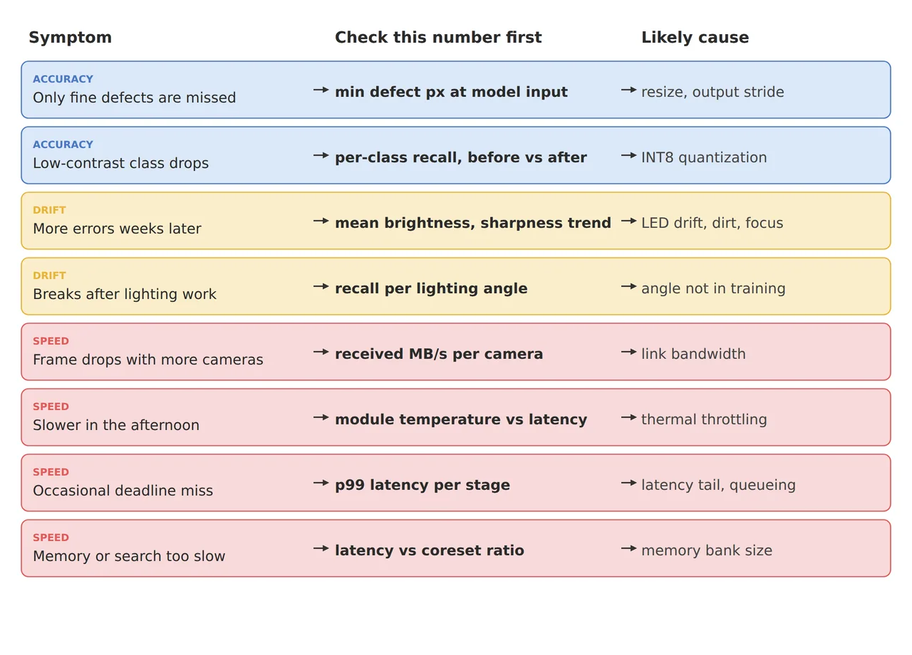
From the top, the figure color-codes accuracy symptoms in blue, drift in yellow and speed in red. Measure one number, and the likely causes on the right narrow to one or two, and only those need following into the detailed articles. To my eye, the middle column is the body of this map.

Category · symptom	Number to check first	Likely cause · basis	In plain words
① Minimum defect size · only fine defects missed	Defect pixels at the model input (3 or more?)	Resizing. 60 μm is 3 px at 20 μm/px, 0.35 px when shrunk to 640 px	In the shrunk image the defect is not even one dot
① Minimum defect size · recall drops only for low-contrast classes	Per-class recall before and after quantization	If highlights stretch the INT8 range, a 0.8 difference becomes 0.8 step	Coarser graduations bury small differences
② Optical setup · change after reinstall or light swap	Measured WD and pixel resolution (20 μm/px held?)	A changed WD changes the pixel count at the model input too	Measure the camera distance again first
② Optical setup · more false and missed calls weeks later	Trend of mean brightness and sharpness	LED decline, dirt, focus drift. A 15% drop reaches the absolute threshold of 170	The input changes first
② Optical setup · collapse after lighting work	Recall per lighting angle	An angle absent from training	Light it has never seen
③ Algorithm · dropped frames after adding cameras	Received MB/s per camera	Three 20 MP cameras at 2 fps need 119.8 MB/s, over about 115 MB/s effective on 1GigE	The road is too narrow
③ Algorithm · slower in the afternoon	Module temperature and inference time series	Clock reduction from heat	It slows as it heats up
③ Algorithm · occasional deadline misses	p99 latency per stage	Latency tail, queueing. 1 in 1,000 means 57.6 parts in 8 hours	The tail hiding behind the average
③ Algorithm · memory or search too slow	Latency and overdetection by coreset ratio	Memory bank size	The album to compare against is too thick

Of the nine lines, retraining is the direct remedy only for lighting-angle generalization and lightweight model design. The rest start from settings and physical quantities outside training: input size, quantization settings, heat, latency, bandwidth and input degradation. That measuring one number per symptom first avoids much of the retraining loop is the conclusion I value most in this map. One number costs less than retraining.

Some lines do not fit this map. On a high-mix line where products and defect types change often, a system that quickly retrains on a few samples may come before cause-checking (few-shot anomaly detection article). In offline sample inspection with plenty of time to spare, the priority of latency and heat drops, and where server inference is possible, the constraints of quantization and heat disappear altogether. On surfaces mixed with reflections, like the gloss of metal terminals, the weight of each cause shifts, and which cause comes first cannot be guaranteed before a sample test.

The habit of stepping from symptom to number is a skill worth learning before model architecture for anyone starting out in edge AI work. From the side that runs the equipment, a system that logs temperature and latency along with brightness from day one cuts the time it takes to solve each problem. This article explains technology and is not investment advice. See our Disclaimer.

Field Note

When a query comes in from the floor, I would ask for three log lines before the model file. Put module temperature, per-stage latency and mean frame brightness on the same time axis, and a heat problem that only shows in the afternoon separates from lighting degradation spread over weeks by its different shape. On a line that went through reinstallation, I measure the WD and pixel resolution again to confirm that a 60 μm scratch still covers three pixels or more at the model input. Only when those three numbers point to the model does retraining get scheduled.

Field Checkpoints

Spread into check items, the field note’s three log lines read as below.

• Do the WD and pixel resolution hold their design values? (if they change after reinstallation or a light swap, so does the pixel count at the model input)
• Does the smallest defect cover three pixels or more at the model input? (shrinking 20 MP to 640 px leaves 60 μm at 0.35 pixel)
• Has per-class recall been compared before and after quantization, and have saturated highlights in the calibration images been checked? (a wider range merges low-contrast signals)
• Are per-stage p99 latency and module temperature logged on the same time axis? (the tail hides behind the average)
• Does each camera’s received bandwidth stay within the link’s effective limit? (three 20 MP cameras at 2 fps need 119.8 MB/s)
• Are input statistics (brightness, sharpness) computed every frame, and are bright defects judged by their ratio to the background? (the ratio holds even when light output falls 15%)

Frequently Asked Questions

When does retraining start?

When a cause remains after checking input size, quantization, heat, latency, bandwidth and input statistics. In particular, if recall per lighting condition drops only under unseen lighting, gathering images under that lighting and retraining is the right remedy.

Does using FP16 instead of INT8 make the problem go away?

16-bit floating point has far finer spacing between representable values, which greatly reduces the risk of merging low-contrast signals, but memory and inference time grow. How fast an edge device handles FP16 varies by device, so measure recall and latency together on the same images and choose.

Doesn’t tiling make inference take too long?

Running 54 tiles one by one multiplies inferences by 54. Tiles can be batched into one pass, or only tiles from areas where defects can occur can be fed in to cut the count, and that trade-off is calculated in the tiled inference article.

Glossary

• [1] Pixel resolution μm/px
  The length on the inspected surface that one pixel covers. Shrinking the image stretches that length by the same factor. ↩
• [2] Recall recall
  The share of real defects that the model catches as defects. Small-defect losses only show when it is read per defect type instead of as an overall average. ↩
• [3] Tiling tiling
  Cutting a large image at full resolution into pieces the size of the model input. It protects small defects at the cost of more inferences. ↩
• [4] Output stride output stride
  How many input pixels one cell of the model output represents. With a stride of 4, one output cell covers 4 × 4 input pixels. ↩
• [5] INT8 quantization INT8 quantization
  Converting a model’s real values into 256 steps of 8-bit integers to lighten the computation. It is like switching to a ruler with coarser marks, so small differences can land on the same mark. ↩
• [6] Calibration calibration
  The step that runs representative images through the model to set value ranges for quantization. Extreme brightness in these images widens the ranges. ↩
• [7] p99 latency 99th percentile
  The value at the 99th percent mark when latencies are lined up from shortest to longest. It exposes the tail that runs late one time in 100 even when the average looks fine. ↩
• [8] Bandwidth MB/s
  The amount of data a link can carry in one second. When several cameras share one link, their total has to fit inside it. ↩
• [9] Memory bank memory bank
  A store of features taken from good-part images, compared against each new image. A larger bank is more accurate but costs memory and search time. ↩

References

• Jacob et al., Quantization and Training of Neural Networks for Efficient Integer-Arithmetic-Only Inference (2017): real value r and integer q related by r = S(q − Z), 8-bit integer-arithmetic inference
• Formulas: resolution after resize = original resolution × (original width ÷ input width), tiles = ⌈width ÷ 640⌉ × ⌈height ÷ 640⌉, asymmetric INT8 step = range ÷ 255, bandwidth = width × height × bytes per pixel × frame rate, deadline misses = parts × miss ratio. Assumptions: 20 MP (5,472 × 3,648 px), 20 μm/px, 1GigE effective 115 MB/s, feature map ranges 0 to 64 and 0 to 256, defect gray 200, background 120, threshold 170

Related reading — It Worked on the Server, So Why Does Accuracy Drop on the Edge? · Where Do Fine Defects Go When You Shrink to 640 × 640? · Why an Average Latency Inside the Deadline Is Not Safe