Adding Reasons to an AOI Defect Call with a Vision Language Model

ALGORITHM

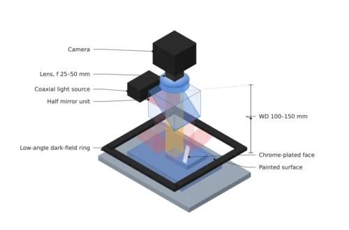
To attach a name and a reason to the single word ‘defective’ that AOI leaves behind, two lighting channels and ten pixels per defect have to be in place before the model.

For a setup that puts a vision language model behind PCB AOI, I calculated the optical evidence the model can rely on and the size of the human review queue.

About 14 min read

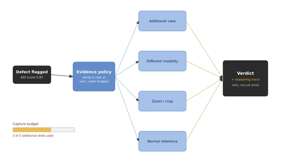
A PCB is up on the AOI (automated optical inspection)¹ screen as defective. All it shows is one coordinate, one crop and an anomaly score² of 0.87. What the next process wants to know, though, is a name more than a score. A solder bridge goes to rework, a missing part goes back to placement, and a single strand of dust just passes.

Without a name, costs arise in two places. People recheck every decision, so the labor saved by automatic inspection comes back, and with no count of how often each defect type occurs, the feedback that fixes the process is cut. That is how a line ends up with the inspection machine running and the yield standing still.

A vision language model (VLM)³ handles images and sentences in the same representation space, so it can take a crop and return the name of the defect along with the reason it sees it that way, in a sentence. What I want to examine sits upstream of the model’s scorecard. All a model can cite as evidence are the differences the camera and lighting have already captured, and what creates those differences, and how much of them, decides whether this setup works.

What a score of 0.87 does not say

An anomaly detector is built to measure how far an image sits from where the normal images gather. 0.87 is that distance squeezed between 0 and 1, so the output has no axis for defect type to begin with. However large the model grows, a single distance does not yield a name.

The old way to get a type name is to label each type and train a multi-class classifier. That path asks for hundreds of labels per type and has to collect them again whenever a new type appears. A vision language model can take type names and descriptions as sentences, so there is room to start with fewer labels, but how few labels reach usable accuracy depends on the product and the defect distribution and cannot be guaranteed before a sample test.

Either way, the reasoning sentence a model returns cannot go beyond the differences held in the input image. If a bridge and a speck of dust are recorded at the same brightness in the crop, the model has no grounds to separate them and may attach a wrong name in a plausible sentence. Light makes the evidence. That is why I put the lighting on the first line of this setup.

Two lights split a bridge from a stray fiber

One PCB mixes four kinds of surface. The green solder mask scatters light fairly evenly, the copper pads and solder are metal and throw light back in one direction like a mirror, and the bodies of chip parts are close to matte. Dust and fiber scraps are diffuse reflection⁴ surfaces that scatter light in every direction. The same defect candidate reacts differently to lighting depending on whether it sits on metal or on a diffuse surface.

Coaxial illumination⁵ sends light down from above along the lens axis, so only metal surfaces close to horizontal return light to the camera. With the lens 166 mm away at F/5.6, the lens entrance subtends a half-angle of 1.5° from the inspected surface, and for a point source a metal surface goes dark once it tilts by a little over 0.8°. A low-angle ring light⁶ does the opposite and lights from a low angle; with the ring 15° above the board, a metal slope tilted 37.5° sends light into the camera. That is why the sloped faces of solder fillets glow under the ring.

Light the two separately and each defect candidate gets two brightness values. A solder bridge is metal, so under the coaxial light only the small flat at its top glints, and under the ring its rounded sides rise as a bright rim. A fiber scrap is a diffuse surface, evenly dim under both lights, and darker under the ring by the amount the light arrives at a slant, about 26 % of straight-down lighting at 15° incidence. The brightness ratio of the two images speaks for the material, and for the model to write the reason ‘a metallic sheen wraps the sides’, both images have to be in its input. I treat this ratio as the first attribute to attach to the model input. The idea of describing a defect as a bundle of such physical attributes and classifying it that way also appears in patents, and the two in the table below are examples.

Patent	Title	Assignee (original)	Priority · granted
US 12,361,531 B2 (published as US 2022/0222806 A1)	Machine learning-based classification of defects in a semiconductor specimen	Applied Materials Israel Ltd.	2019-05-22 · 2025-07-15
US 10,599,951 B2	Training a neural network for defect detection in low resolution images	KLA Corp (KLA-Tencor Corp)	2018-03-28 · 2020-03-24

The Applied Materials Israel patent trains a machine learning model to output, for each defect, a vector bundling several physical attribute values that help separate the classes, and classifies by matching that vector against the attribute sets defined for each class. A value such as the brightness ratio of the two lights can be a candidate for such an attribute. The KLA patent trains a network for low-resolution inspection images using defect images synthesized by a high-resolution network, so defects can be found faster than with high-resolution imaging. This division of labor, finding coarsely and naming finely, is where the next calculation starts.

A 32.8 mm field that puts an 80 μm bridge on ten pixels

To attach a name, the shape of the defect has to be readable inside the crop. My rule is 8 μm/px, which spreads an 80 μm bridge across ten pixels, and with a 12 MP-class color sensor of 4,096 × 3,000 px and 3.45 μm pixels (assumed) that gives a 32.8 × 24.0 mm field of view at 0.431 magnification. With a 50 mm lens the WD⁷ from lens to board is about 166 mm, so the first check is whether there is room to fit both the coaxial light and the low-angle ring.

The Bayer pattern⁸ of a color sensor takes red and blue on only one pixel in every two across and down, so in color the spacing widens to 16 μm. An 80 μm bridge gets about five color samples, enough to separate the silver of solder from the copper color of the pads, but the edge shape of the bridge is safer to read from the brightness channel. A 60 μm particle covers 7.5 pixels, and a part shifted 150 μm from its reference position shows up 18.8 pixels off.

The crop size comes out of the same calculation. A 256 × 256 px crop is a 2.05 mm square on the board, so a 0402 chip at 1.0 × 0.5 mm or a 0603 chip at 1.6 × 0.8 mm fits in one crop along with the surrounding pads, and four leads at 0.5 mm pitch fit as well. Only when the model sees the neighboring leads, beyond the defect alone, does the reason ‘metal joining two leads’ hold.

Covering a 100 × 80 mm board with this field, with neighboring frames overlapping by 10 %, takes 4 frames across and 4 down, 16 in all. Shooting both lights alternately in every frame still makes only 32 images, and at 40 ms per image that is 1.28 seconds. If the model takes 0.5 seconds to read one candidate, a board with three candidates adds 1.5 seconds. Once both lights are captured from the start, choosing which evidence to look at next stops being a question of shooting again and becomes a question of what to feed the model.

Set side by side, the numbers show where the cost lies. Capture is done in 1.28 seconds per board, but model inference and human review grow in proportion to the number of candidates. The operating numbers are therefore set by how many candidates come out and how many of them a person looks at.

The human review queue starts at 130 items an hour

The starting point is to send low-confidence items to a person. Inspecting 180 boards an hour, with three candidates per board and, at first, 20 % of them below a confidence of 0.6 (assumed), a person has 108 items an hour to look at. Add an audit of 21.6 items drawn at random from 5 % of the high-confidence items and it comes to about 130, which at 10 seconds each ties up 21.6 minutes every hour, a little over a third of one person. That is no small share.

The random audit is there because looking only at low-confidence items never exposes the ‘confidently wrong’ decisions. The human review queue is a sieve that collects only hard cases, so accuracy measured from it differs from the accuracy of the model as a whole. The figure of 0.6 also means different things for different models, so confidence calibration⁹, which matches the actual hit rate in each confidence band against the audit results, has to go with it. The review results are not thrown away but go back into retraining, and the figure is a concept diagram of that loop.

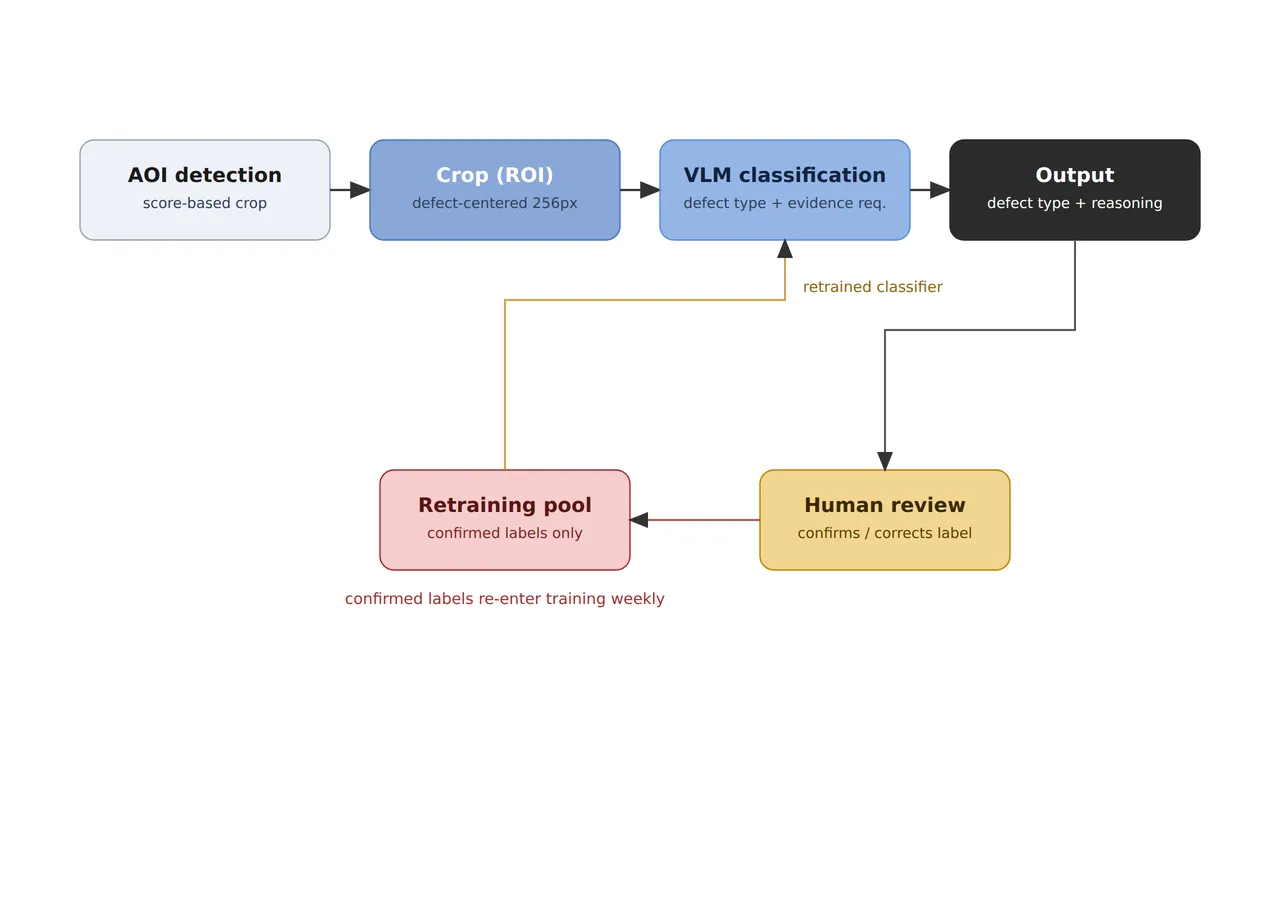
The lower loop, where only labels a person has confirmed or corrected enter the retraining pool and return to the classifier each week, is how this setup raises its accuracy. The speed of that loop can be calculated too. Running 16 hours a day, a little over 2,070 confirmed labels pile up daily, and a rare type that makes up 2 % gets 41 a day, so collecting 300 takes a little over a week. Measuring 90 % accuracy on 300 items gives a 95 % confidence interval¹⁰ of ±3.4 points, and on 50 items ±8.3 points, so the accuracy of a rare type is hard to state in numbers during the first week.

So I recommend writing three numbers into the specification in place of a single target accuracy: the accuracy in the first week, the number of confirmed labels added per day, and the date by which 300 items per type have been collected. Only with these three numbers is there an answer to when human review can be reduced.

Carrying the rationale into the specification

Gathering the calculations into one table puts the reasons the model will give on the same line as the hardware that creates them. The middle rows of the table say that the two lighting channels and the evidence budget come as a pair.

Item	Value	Condition · basis	In plain words
① Minimum defect size (μm)	Solder bridge 80 μm wide, surface particle 60 μm across, part shift 150 μm	10 · 7.5 · 18.8 pixels at 8 μm/px. Color samples every 16 μm (Bayer)	Shape is read from brightness, color only coarsely
② Lighting	Coaxial + low-angle ring (15° elevation), two channels lit independently, uniformity within ±5 % per channel	A 15° ring lights metal slopes tilted 37.5°. The brightness ratio of the two channels is a material attribute	Metal and dust look different under the two lights
② Camera · lens · WD	12 MP-class color (4,096 × 3,000 px, 3.45 μm assumed), 50 mm F/5.6, field of view 32.8 × 24.0 mm	WD of about 166 mm must be secured (thin-lens approximation), interference with both light housings measured	Both lights have to fit under the lens
③ Algorithm parameters	AOI detection → 256 × 256 px crop (2.05 mm) + both lighting images + one normal reference → VLM type · reason	Human review below 0.6 confidence (reset after calibration), random audit of 5 % of high-confidence items, weekly retraining	Confidently wrong cases are found by the audit

The cell in this table most likely to give way first is the lighting channel in ②. With only a coaxial light, the evidence the model can choose is limited to zooming in and the normal reference, so candidates of similar shape, such as a bridge and a metallic particle, do not separate even in sentences. I would reopen the optical setup at the moment the algorithm is brought in. Per-channel uniformity of ±5 % is held for the same reason. As long as the brightness ratio of the two channels serves as a material attribute, one channel brightening by 5 % shifts the whole ratio by 5 %.

There are clearly lines where this setup does not fit. If the defect types are fixed at two or three and new types hardly ever appear, collecting enough labels per type and going with a multi-class classifier is lighter in both inference time and operation. If the tact time is tight on the scale of tens of milliseconds, separating type classification into batch processing after inspection is more realistic, and on a line where no one reads the decision rationale the sentences are worth less. How often the model’s reasoning sentences are actually right on images that mix highly glossy solder with reflective pads cannot be guaranteed before a sample test.

Choosing the model is the algorithm engineer’s job, but the lighting rows and the operating rows of this table have to be set together with equipment and quality staff. Whether a third of a person can be assigned to the review queue, and whether the accuracy of rare types can be seen after a week, set the schedule for introduction. When budgeting for it, check whether the audit rate and the label return path are written into the specification, more than whether it carries the name ‘AI classification’. This article explains technology and is not investment advice. See our Disclaimer.

Field Note

To attach a vision language model to a line where AOI only leaves the word ‘defective’, I would put the evidence region ahead of the reasoning sentence. I would sample about 50 items from the review queue to check whether the region the model points to matches the actual defect location, and if many are off, I would treat the output as clouding rework decisions however plausible the sentences are. Next I would split the same candidates into runs with only the coaxial image and runs with both lighting images and see whether the name changes. If it does not, the model is not using the second light as evidence, and I would revisit the input configuration.

Field Checkpoints

Once the evidence region and the input configuration have been checked, only the questions below remain.

• Is a WD of about 166 mm from lens to board (50 mm lens, 32.8 mm field of view) actually available with both the coaxial light and the low-angle ring fitted? (a distance measured inside the equipment in place of a drawing value)
• Does the hardware actually offer at least two lighting channels for the model to choose from? (with coaxial alone there is no basis for naming the material)
• Does an 80 μm bridge span ten pixels, and does one crop include the neighboring leads? (256 px = 2.05 mm)
• Is the uniformity within ±5 % per channel, and has the brightness ratio of the two channels been referenced on good parts?
• Has the 0.6 confidence been calibrated against the actual hit rate using audit results? (0.6 means different things for different models)
• Are the 5 % random audit of high-confidence decisions and the staffing of the review queue (a little over a third of a person) defined?
• Do review results flow into the retraining pool automatically, and is the date by which 300 items per type are collected written into the specification?

Frequently Asked Questions

Can the vision language model take over AOI detection as well?

Not in this setup. Covering one 12 MP frame entirely in 256 px pieces takes 192 crops, and the 16 frames of a board take 3,072, which at 0.5 seconds each comes to 25.6 minutes. That is over a thousand times longer than the 1.5 seconds spent reading three candidates. Leaving detection to a fast anomaly detector and attaching the model only to candidates is the division of labor that keeps the numbers at 1.28 seconds of capture and 1.5 seconds of inference.

Why include one normal reference image?

Placing a normal crop of the same part position alongside lets the model see by comparison what should be at that spot. Defects where a part is missing or its polarity is reversed are hard to argue from the defect crop alone. The reference also has to be shot with the same two lighting channels for the brightness-ratio comparison to hold.

Glossary

• [1] AOI automated optical inspection
  Inspection equipment that photographs boards or parts with cameras and lighting and finds defect candidates automatically. It usually outputs defect positions and scores. ↩
• [2] Anomaly score anomaly score
  A value expressing how far an inspection image lies from the distribution of normal images. A large value only means something is unusual; it does not say what. ↩
• [3] Vision language model VLM
  A model that takes images and text together and answers about the image in sentences. In inspection it can give the defect name and the reason in a sentence. ↩
• [4] Diffuse reflection diffuse reflection
  Reflection in which light scatters in every direction from a rough surface. Brightness changes only gently when the lighting direction changes. ↩
• [5] Coaxial illumination coaxial illumination
  Lighting that bends light with a half mirror so it comes down along the same axis as the lens. Flat metal surfaces look bright and tilted ones dark. ↩
• [6] Low-angle ring light low-angle ring light
  Ring-shaped lighting that shines from a low angle close to the inspected surface. Slopes, edges and anything raised light up. ↩
• [7] WD working distance
  The distance from the lens to the surface being inspected. The value in the text uses a thin-lens approximation measured from the lens center. ↩
• [8] Bayer pattern Bayer pattern
  An arrangement that places one of red, green or blue filters on each pixel of a color sensor in a checkerboard. Looking at a single color, the pixel spacing widens. ↩
• [9] Confidence calibration confidence calibration
  Adjusting the confidence a model reports so it matches the actual hit rate. It checks whether decisions given at 0.8 confidence are in fact right 80 % of the time. ↩
• [10] Confidence interval confidence interval
  The range within which a value measured on a sample is expected to hold the true value. It widens as the sample gets smaller. ↩

References

• Applied Materials Israel Ltd., US patent US12361531B2, Machine learning-based classification of defects in a semiconductor specimen (published as US20220222806A1; priority May 22, 2019; filed March 24, 2020; granted July 15, 2025)
• KLA Corp (original assignee KLA-Tencor Corp), US patent US10599951B2, Training a neural network for defect detection in low resolution images (priority March 28, 2018; filed March 25, 2019; granted March 24, 2020)
• Formulas: field of view = pixel count × pixel resolution, magnification = pixel size ÷ pixel resolution, WD ≈ f × (1 + 1/m), lens entrance half-angle = atan(aperture diameter ÷ 2 ÷ WD), metal slope matched to the ring = (90° − ring elevation) ÷ 2, irradiance ratio on a diffuse surface = sin(elevation of incidence), Bayer color spacing = 2 × pixel resolution, frames = ⌈board width ÷ (FOV × 0.9)⌉ × ⌈board height ÷ (FOV × 0.9)⌉, human reviews = boards × candidates × (below-gate share + (1 − below-gate share) × audit share), confidence half-width = 1.96 × √(p(1 − p) ÷ n)

Related reading — Overdetection or Missed Detection, Which One Costs More? · Deep Learning vs. Rule-Based Algorithms, When to Use Which · When the Light Dims by 5 %, How Many Good Pixels Turn Into Defects?